Lattice-Based Training of Bottleneck Feature Extraction Neural Networks Matthias Paulik Cisco Systems Inc., USA
[email protected]
1. Introduction Bottleneck (BN) features [1] are a popular method for improving the accuracy of standard GMM-HMM automatic speech recognition systems [2, 3, 4, 5, 6, 7]. Bottleneck feature extraction (FE) networks are typically constructed as follows. First, a multi-layer neural network (NN) with a small dimensional middle layer (hence the name “bottleneck”) is created and trained to discriminate phonetic states, using frame-based cross-entropy error back-propagation. Input to the NN are standard acoustic features, such as MFCC, PLP or TRAPs [8] features. The NN is usually trained to predict mono-phone states, since finer targets require more training data and more complex classifiers [6]. Training typically relies on “hard” labels, obtained by forcealigning the training utterances with a standard GMM-HMM system. After training, the layers after the BN layer are removed. The outputs of the neurons in the BN layer now serve as acoustic features for training a standard GMM-HMM system. BN features are frequently used together with standard features by simply concatenating BN feature vectors with standard feature vectors. In this paper, we propose to extend the standard recipe for training BN feature extraction networks. In particular, we investigate if it is possible to train a BN FE network in a more targeted manner for its intended use in GMM-HMM based ASR. In some sense, we try to jointly train the GMM acoustic model (AM) and the feature extraction network. Hence, our approach bears similarities to work described in [9], where the parameters of the feature transformations are optimized simultaneously with the HMM parameters according to a discriminative objective criterion. In our work, we construct a “joint” neural network that includes both, AM and FE component. We training this joint network using a lattice-based sequence classification criterion [10]. After training, the GMM component
input layer affine transforma,on
3496 x 368
hidden layer (sigmoid) affine transforma,on
30 x 3496
bo5leneck Removed a7er training
This paper investigates a method for training bottleneck (BN) features in a more targeted manner for their intended use in GMM-HMM based ASR. Our approach adds a GMM acoustic model activation layer to a standard BN feature extraction (FE) neural network and performs lattice-based MMI training on the resulting network. After training, the network is reverted back into a working BN FE network by removing the GMM activation layer, and we then train a GMM system on top of the bottleneck features in the normal way. Our results show that this approach can significantly improve recognition accuracy when compared to a baseline system that uses standard BN features. Further, we show that our approach can be used to perform unsupervised speaker adaptation, yielding significantly improved results compared to global cMLLR adaptation. Index Terms: speech recognition, bottleneck features, neural networks, sequence based training criteria
Baseline BN feature extrac,on NN
Abstract
affine transforma,on
3496 x 30
hidden layer (sigmoid) affine transforma,on
144 x 3496
so8max output layer Error computa,on: frame-‐based cross-‐entropy
Figure 1: Baseline Bottleneck Neural Network. is once again removed from the network to obtain a working BN FE network. In this work, we do not update the parameters of the GMM components when back-propagating in the described joint network. However, we investigate the reestimation of the GMM acoustic model based on the new BN features, using standard Expectation Maximization (EM) training. We consider Viterbi based Maximum Likelihood (ML) training as well as model and feature-space discriminative training based on boosted Maximum Mutual Information (bMMI, fbMMI) [11, 12]. We also investigate the effectiveness of our approach for unsupervised speaker adaptation and compare it to global cMLLR [13] speaker adaptation.
2. Baseline BN FE Neural Network Figure 1 shows our baseline BN feature extraction network. The network has the same architecture as the baseline BN network described in [4]. The input features to the network are based on TRAPs. The training network has 5 layers; input layer (368), sigmoid hidden layer (3496), bottleneck layer (30), another sigmoid hidden layer (3496) and finally a softmax output layer (144). The numbers in braces indicate the dimension of the respective layers. The individual layers are connected by affine transformations: y = Ax + b. The elements of the transformation matrix A and the bias term b correspond to the updateable weights of the NN. The input to the network is based on 23 short-term mel-scaled log-energy trajectories. We obtain the trajectories by concatenating 31 frames, weighted by the Hamming window and projected onto the first 16 Discrete Cosine Transform bases. We apply global mean normalization before feeding these 23 × 16 = 368 dimensional features to the network. The 144 targets correspond to the mono-phone states of 43 speech phones, with 3 states each and 3 silence/noise phones, with 5 states each. Training labels are obtained by mapping the alignments from a tri-phone GMM-HMM system to the respec-
P → → → log(pdf (− x )) = log( i wi Gi (− x;− µi , Σ i )
Removed a;er training
Proposed JT-‐BN feature extrac,on NN
input layer affine transforma,on
3496 x 368
hidden layer (sigmoid) affine transforma,on
30 x 3496
Given diagonal covariance matrices, each multi-variate Gaussian Gi can be computed from the product of the univariate Gaussians Nid Q → 2 Gi (− x ) = d Nid (xd ; µid , σid )
bo5leneck mean normaliza,on (per uMerance) affine transforma,on*
30 x 30
GMM layer
n GMMs
Error computa,on: laGce-‐based MMI *: before the first weight update, the last affine transform is equivalent to the combined, non-‐reducing LDA+MLLT matrix
Figure 2: Proposed Joint Neural Network. tive mono-phone states. Training is done frame based in minibatches of 256, using the combination of softmax plus crossentropy error criterion.
3. Joint Neural Network 3.1. Network Construction Figure 2. shows the joint NN used to further train the BN features towards a specific GMM-HMM system. The joint NN is a combination of (A) the original BN feature extraction network; and (B) components of the GMM-HMM that were trained based on the original BN features. We add those components of the GMM-HMM system that ensure that the joint network now produces the per-frame log-likelihoods of all GMM-HMM acoustic states (senones). Our GMM-HMM system transforms the mean normalized BN features by applying a non-reducing transformation that results from computing and combining LDA and MLLR transforms. Hence we add a “mean normalization component” as well as an updatable affine transformation that corresponds to the LDA+MLLR transformation matrix. The mean normalization component subtracts the means of the current data batch1 from the individual BN layer outputs. After applying the LDA+MLLT affine transformation, we have a 30 dimensional feature vector that we feed to each GMM component in the GMM layer. In this work, we do not allow updates to the parameters of the GMMs via back-propagation. However, we allow updates to the LDA+MLLR affine transformation. It should be noted that all components of the bias term b are set to 0 when we first construct the joint network, but b is typically non-zero after back-propagation. After training the described joint network, we remove the GMM layer. However, as indicated in Figure 2, we keep the mean normalization and the final affine transformation in place when we compute BN features with this network. 3.2. Training the Joint Neural Network In order to back-propagate the error through the proposed joint network, we have to compute the derivative of the GMM components with respect to the 30 data dimensions. Since we only make use of diagonal covariances, computation of the derivative is straightforward. The log-likelihood of each GMM component is given as 1 This corresponds to per-utterance mean normalization, since we back-propagate each training utterance.
with 2 Nid (xd ; µid , σid )=
√ 1 e 2πσid
−
(xd −µid )2 2σ 2 id
When computing the derivative of Gi with respect to xd , we only have to compute the derivate of Nid , since all other multiplicative factors are being treated as constants. The derivative of Nid is Nid itself, multiplied by a factor Fid dNid dxd
= Fid Nid with Fid =
µid −xd 2 σid
Putting everything together, we now see that the derivative → of pdf (− x ) with respect to xd can be computed by multiplying the likelihoods of its individual multivariate Gaussians by their respective factors Fid . Caching the likelihoods of the mixture components when they are computed in the forward pass allows for an efficient computation of the derivative during back-propagation. Finally, we should not forget that we are actually working with log-likelihoods. The derivative of log(g(x)) is g 0 (x)/(g(x). Hence, to arrive a the final result, → we have to divide the derivative of pdf (− x ) with respect to xd − → by the orginial likelihood pdf ( x ). We train the joint neural network using a lattice-based sequence classification criterion [10]. As described in [10], the gradient of any sequence classification error function Lseq (e.g. the negative of the MMI objective function) with respect to state log-likelihoods lrt (i) of state i at time t and given same r can be computed based on the expected state occupancies γrt (i): dLseq dlrt (i)
DEN NUM = k(γrt (i) − γrt (i))
The expected state occupancies are computed via forwardbackward passes over the numerator and denominator lattices; k refers to the acoustic scaling factor. Our state log-likelihoods are normalized by the prior probability p(i) of state i: lrt (i) = log yrt (i) − log p(i). According to the chain rule, we therefore need to compute: dLseq dyrt (i)
=k
DEN NUM γrt (i)−γrt (i) yrt (i)
Training is accomplished with the help of the Kaldi Speech Recognition toolkit [14], which includes binaries for lattice-based MMI back-propagation. As a reminder, the MMI objective function is: OBJM M I =
R P r=1
p(Xr |Msr )k P (sr ) k s p(Xr |Ms ) P (s)
log P
where Xr are the training utterances, Ms is the HMM sequence corresponding to a sentence s and sr is the reference transcription. We have extended Kaldi accordingly to support the construction and back-propagation of the described joint neural network. We plan to release our extension to Kaldi.
4. Overall Training Recipe Our overall training recipe is as follows: 1. 2. 3. 4. 5.
Build MFCC GMM-HMM baseline systems Train BN network, convert to FE network Build BN GMM-HMM baseline systems Train joint neural network, convert to FE network Build final JT-BN GMM-HMM systems
By default, we train tri-phone based systems. First, we estimate an ML trained AM via several iterations of Viterbi. We then further refine the AM by n iterations of feature space bMMI (fbMMI) training, followed by n iterations of model space bMMI training. Finally, we re-create the denominator lattices and add several more iterations of bMMI. It should be noted that we did not observe any further improvements for any of the 3 types of GMM-HMM systems by adding any more training iterations or by re-estimating the denominator lattices once more. The systems of step 1 and 3 both estimate combined LDA and MLLT matrices in their ML training step. For the MFCC system, we splice 9 frames and the LDA transform reduces the dimensionality of the spliced feature vector to 40. The LDA transform of the BN system in step 3 is non-reducing, i.e. the feature dimension is 30. The BN systems of step 5 directly use the 30 dimensional features produced by our proposed BN FE network. That is, no additional feature transformation matrices are computed for the systems of step 5. We boot-strap training of all our ASR systems (step 1,3 and 5) with one common set of alignments obtained from a legacy system. We found that training the joint NN works best if we use a GMM layer that corresponds to the ML trained AM, as opposed to using a discriminatively trained AM. Further, we observed that when using the proposed jointly trained BN features in step 5, it is best to re-train the AM, starting with the ML build. It should be noted that alternatively, one could simply use the ML AM from the BN-GMM system of step 3 as a starting point. While re-training the AM in step 5 results in slightly worse word error rates (WERs) in the ML stage itself, we see better results in the subsequent discriminative AM training steps.
5. Experiments 5.1. Data and Language Model The AM training data consists of 30h worth of accurately labeled Cisco Television (CTV) data plus several hundred hours of loosely transcribed Cisco meeting data (please see Section 5.2 for more details). The language model (LM) training data comprises 560 million running words over a 58k vocabulary. The decoding dictionary has 64k entries. A detailed description of our loosely transcribed corpus and how we leverage these transcriptions for AM training, as well as a more detailed description of the LM training data can be found in [15]. We make use of one development (dev) set and one test set. The dev set consists of 2h of accurately transcribed CTV data. The test set consists of 7h of accurately transcribed Cisco meeting data. We apply a 2-gram LM during decoding. Table 1 lists the 2-gram LM perplexity (PPL) as well as the out-of-vocabulary (OOV) rates for both sets. The LM is trained with the SRI LM Table 1: Development and test set statistics. Duration 2-PPL OOV Dev 2 hours 255 0.93% Test 7 hours 213 1.70%
Table 2: Dev set WERs of pilot system. AM train. crit. MFCC BN JT-BN ML 40.3 36.5 32.9 (32.5) fbMMI 36.4 32.2 29.9 bMMI 31.8 29.3 27.3 lats & bMMI 30.0 27.6 26.4 toolkit [16], all other system components are trained with the Kaldi Speech Recogntion toolkit [14]. 5.2. ASR Systems We report results for three differently sized ASR systems. We develop our training recipe on a very small “pilot system”, trained on 30h of CTV data. The AM of this pilot system has 235 clustered tri-phone states with 4k Gaussians total. An “intermediate system”, trained on 100h of data that was randomly picked from all available AM training data is used to confirm our training recipe. The AM of the intermediate system has 1674 clustered tri-phone states and in total 32k Gaussians. Finally, we report some preliminary results on a “large system”, trained on 300h worth of data, again picked randomly from our larger pool of training data. The AM of the large system has 5095 clustered tri-phone states and 96k Gaussians total. 5.3. Results Table 2 lists the WERs of our pilot system on the dev set. By switching from 40 dimensional MFCC features to 30 dimensional BN features, which are based on TRAPs, we already observe significant gains in accuracy. By performing the described joint training of BN features, denoted in the table by JT-BN, we observe another signifiant gain. First, it should be noted that by switching to JT-BN features, we see a reduction in WER that is in the same order of magnitude as for feature space bMMI training; 32.2% vs. 32.5%. The number shown in brackets corresponds to the decoding results when using JT-BN features in combination with the ML trained AM of the BN system. ML re-training the AM using JT-BN features results in a slight increase in WER to 32.9%. Despite this increase in WER, and as already mentioned in Section 4, the subsequent discriminative AM training benefits from such a re-training. Hence, all other numbers reported in the last column of Table 2 have this re-estimated ML AM as a starting point. Training of the joint NN is based on the same lattices used for performing feature space bMMI training on the BN system. However, discriminative AM training in step 5 computes its own set of lattices. One could argue that the re-computation of lattices may be responsible for the observed performance gains. For this reason, we re-generate the lattices and repeat model space bMMI training until we observe no further gains. The last row of Table 2 shows the results obtained when regenerating the lattices once more and adding another round of bMMI training iterations. Re-generating the lattices more than once does not lead to any further improvements. Tables 3 and 4 list the dev set and test set WERs of our intermediate systems. The results in the first four data rows correspond to the results computed for the pilot system, i.e. using a speaker independent single-pass system. The index shown for the label JT-BNi1p6 denotes the training iteration of the joint NN that was available at the time of writing. We write intermediate results every 10h worth of back-propagated training utterances. The index shown tells us that we are still in the first iteration of going through all training utterances and we have observed 60h worth
Table 3: Dev set WERs of intermediate system. AM train. crit. MFCC BN JT-BNi1p6 ML 30.3 27.0 25.6 (25.0) fbMMI 28.8 25.3 24.4 bMMI 25.3 22.4 21.8 lats & bMMI 24.9 22.1 21.3 cMLLR 22.5 19.9 19.4 Table 4: Test set WERs of intermediate system. AM train. crit. MFCC BN JT-BNi1p6 ML 41.0 37.5 35.7 (34.6) fbMMI 39.1 34.9 33.9 bMMI 34.4 30.9 29.9 lats & bMMI 33.6 30.0 29.2 cMLLR 30.9 27.5 27.4 of data so far. As can be seen, the WER reductions are similar to what we had observed on our pilot system. The results in the last data row are obtained by applying unsupervised speaker adaptation via global cMLLR. We perform acoustic re-scoring of the lattices from the first pass, using the same AM, but cMLLR transformed features. The results after cMLLR are inconsistent; on the dev set, the JT-BN features still outperform standard BN features, however, the gain in performance is slightly reduced. On the test set, the performance gain achieved by using JT-BN features vanishes after cMLLR. We discuss this issue in more detail in Section 6 and propose a possible solution. We are interested in the question if a joint FE network that was trained with a smaller amount of data and with a GMM layer stemming from a different, smaller AM can help improve the performance of a larger AM. To this end, we take the JT-BN features stemming from our intermediate system experiments, and apply them to our large system. Table 5 summarizes the results on our test set for this experiment. The last data row list the WER after applying global cMLLR adaptation. The gain in transcription accuracy compared to using standard BN features is again strongly reduced after applying cMLLR. However, the observed reduction in WER from 25.9% for the standard BN features after cMLLR to 25.7% for the JT-BN features after cMLLR is statistically significant at a level of p = 0.001.
6. Discussion and Future Work We can identify several reasons that most likely contribute to the observed performance gains. First, the joint NN is trained to predict tri-phone states. It has already been shown in [7] that better BN features can be obtained by training towards senones rather than mono-phone states. Yu et al. [7] report reductions in sentence error rate of up to 2.5% relative by switching from mono-phone to senone targets. Second, the GMM layer corresponds to a ML trained AM. Hence, when we back-propagate the error through the network, we are in some sense trying to correct the errors made by the AM. Third, we train the joint NN using a sequence based classification criteria [10], instead of using frame-based training. And fourth, our recipe replaces the combined LDA+MLLT transform with an affine transform that is trained as part of the joint NN. The performance gains from our JT-BN features, compared to standard BN features, are strongly reduced after applying global cMLLR. We believe that this effect can be countered by applying discriminative speaker adaptation. One possible solution could be to train the joint NN for each speaker cluster for a few
Table 5: Test set WERs of large system. The JT-BN∗ features are identical to the ones estimated for the intermediate system. MFCC BN JT-BN∗i1p6 1st pass 30.4 28.4 27.5 cMLLR 27.8 25.9 25.7 Table 6: JT-NN based unsupervised speaker adaptation. Dev Test BN JT-BN BN JT-BN baseline 27.0 25.0 37.5 34.6 cMLLR 25.3 23.8 35.3 33.1 JT-NN adapt n/a 23.2 n/a 32.1 iterations, using the results from the first pass as ground truth. Table 6 lists some preliminary results for this approach. These experiments are conducted with the ML-AM that was trained using standard BN features. The first data row corresponds to the results shown in the first data rows of Tables 3 and 4. The second data row shows the results after re-scoring the baseline lattices with cMLLR transformed features. The last data row shows the results after re-scoring the baseline lattices with JTBN features that are obtained after having trained joint NNs for each speaker cluster, using the first best path of the lattice as ground truth. The results show that the proposed approach for unsupervised speaker adaptation is feasible and outperforms global cMLLR significantly. Our experiments have been limited to a BN FE network with only one single hidden layer and with a fixed GMM layer. It is conceivable that better results can be achieved with larger and deeper NNs and a GMM layer that allows updates to its parameters. In this context, it should be noted that computing the derivatives of the GMM components with respect to their means and co-variances leads to similar mutliplicative factors Fid as discussed in Section 3.2. However, training via gradient descent is notoriously slow and it is questionable if such an approach would yield significantly better results than first estimating the joint NN and then training the AM via EM. Repeating aforementioned two steps may also lead to further improvements.
7. Summary We proposed a novel technique for training bottleneck feature extraction neural networks in a more targeted manner towards their use in GMM-HMM based speech recognition. Our approach allows to train BN FE networks using lattice-based sequence classification criteria by essentially interpreting the combination of standard BN FE network and GMM-HMM acoustic model as a “joint neural network”. We have shown that our approach can yield significant reductions in word error rate compared to using standard BN features. In particular, when applying our approach to a ML trained acoustic model, we observe WER reductions that are similar to the reductions achieved by feature space bMMI [12]. Further, we have demonstrated that our approach can be used to perform unsupervised speaker adaptation, yielding significantly improved results compared to global cMLLR adaptation.
8. Acknowledgements Special thanks go to K. Vesely for providing the authors with an early version of his code for NN MMI training. Thanks also go to D. Povey for proof-reading and providing valuable feedback.
9. References [1]
Fontaine, V., Ris, C. and Boite, J.-M., “Nonlinear discriminant analysis for improved speech recognition”, in Proc. Eurospeech, 1997.
[2]
Grezl, F., Karafiat, M., Kontar, S. and Cernocky, J., “Probabilistic and bottle-neck features for LVCSR of meetings,” in Proc. ICASSP 2007.
[3]
Fousek, P. , Lamel, L. and Gauvain, J. , “Transcribing Broadcast Data Using MLP Features”, in Proc. Interspeech, 2008.
[4]
Grezl, F., Karafiat and M., Burget, L., “Investigation into bottleneck features for meeting speech recognition”, in Proc. Interspeech, 2009.
[5]
Metze, F., Hsiao, R. , Jin, Q., Nallasamy, U. and Schultz, T. “The 2010 CMU GALE Speech-to-Text System”, in Proc. Interspeech, 2010.
[6]
Grezl, F. and Fousek, P., “Optimizing bottle-neck features for LVCSR”. in Proc. ICASSP, 2006.
[7]
Dong Yu, Michael L. Seltzer, “Improved Bottleneck Features Using Pretrained Deep Neural Networks”, in Proc. Interspeech, 2011.
[8]
Hermansky, H. and Sharma, S., “Temporal patterns (TRAPS) in ASR of noisy speech”, in Proc. ICASSP, 1997.
[9]
Valtcho, V., “Discriminative Methods in HMM-based Speech Recognition”, PhD thesis, University of Cambridge, 1995.
[10] Kingsbury, B., “Lattice-based Optimization of Sequence Classification Criteria for Neural-Network Acoustic Modeling”, in Proc. ICASSP, 2009. [11] Woodland, P.C. and Povey, D., “Large scale discriminative training of hidden Markov models for speech recognition”, Computer Speech and Language, vol. 16 , pp. 25-47, 2002. [12] Povey, D., Kanevsky, D., Kingsbury, B., Ramabhadran, B., Saon, G. and Visweswariah, K., “Boosted MMI for Model and Feature Space Discriminative Training”, in Proc. ICASSP, 2008. [13] Gales, M. J. F, “Maximum likelihood linear transformations for HMM-based speech recognition”, Computer Speech and Language, vol. 12, pp. 7598, 1998. [14] Povey, D., Ghoshal, A., Boulianne, G., Burget, L., Glembek, O., Goel, N., Hannemann, M., Motlicek, P., Qian, Y., Schwarz, P., Silovsky, J., Stemmer, G. and Vesely, K., “The Kaldi Speech Recognition Toolkit”, in Proc. ASRU, 2011. [15] Paulik, M. and Panchapagesan, P. “Leveraging Large Amounts of Loosely Transcribed Corporate Videos for Acoustic Model Training”, in Proc. ASRU, 2011. [16] Stolcke, A., “SRILM - An extensible language modeling toolkit”, in Proc. ICSLP, 2002.