Learning Beyond Finite Memory in Recurrent Networks Of Spiking

Learning Beyond Finite Memory in Recurrent Networks Of Spiking Neurons Peter Tiˇ no Ashley J.S Mills School Of Computer Science University Of Birmingham Birmingham B15 2TT, UK

Abstract We investigate possibilities of inducing temporal structures without fading memory in recurrent networks of spiking neurons strictly operating in the pulse-coding regime. We extend the existing gradient-based algorithm for training feed-forward spiking neuron networks, SpikeProp (Bohte, Kok & La Poutr´e, 2002), to recurrent network topologies, so that temporal dependencies in the input stream are taken into account. It is shown that temporal structures with unbounded input memory specified by simple Moore machines (MM) can be induced by recurrent spiking neuron networks (RSNN). The networks are able to discover pulse-coded representations of abstract information processing states coding potentially unbounded histories of processed inputs. We show that it is often possible to extract from trained RSNN the target MM by grouping together similar spike trains appearing in the recurrent layer. Even when the target MM was not perfectly induced in a RSNN, the extraction procedure was able to reveal weaknesses of the induced mechanism and the extent to which the target machine had been learned.

1

Introduction

A considerable amount of work has been devoted to studying computations on time series in a variety of connectionist models, most prominently in models with feedback delay connections between the neural units. Such models are commonly referred to as recurrent neural networks (RNNs). Feedback connections endow RNNs with a form of ‘neural memory’ that makes them (theoretically) capable of processing time structures over arbitrarily long time spans. However, even though RNNs are capable of simulating Turing machines (Siegelmann & Sontag, 1995), induction of nontrivial temporal structures beyond finite memory can be problematic (Bengio, Frasconi & Simard, 1993). Finite state machines

1

(FSMs) and automata constitute a simple, yet well established and easy to analyze framework for describing temporal structures that go beyond finite memory relationships. In general, for a finite description of the string mapping realized by an FSM, one needs a notion of an abstract information processing state that can encapsulate histories of processed strings of arbitrary finite length. Indeed, FSMs have been a popular benchmark in the recurrent network community and there is a huge amount of literature dealing with empirical and theoretical aspects of learning finite state machines/automata in RNNs (e.g. ˇ (Cleeremans, Servan-Schreiber & McClelland, 1989; Giles et al., 1992; Tiˇ no & Sajda, 1995; Frasconi et al., 1996; Omlin & Giles, 1996; Casey, 1996; Tiˇ no et al., 1998)). However, the RNNs under consideration have been based on traditional artificial neural network models that describe neural activity in terms of rates of spikes1 produced by individual neurons (rate coding). It remains controversial whether, when describing computations performed by a real biological system, one can abstract from the individual spikes and consider only macroscopic quantities, such as the number of spikes emitted by a single neuron (or a population of neurons) per time interval. Several models of spiking neurons, where the input and output information is coded in terms of exact timings of individual spikes (pulse coding) have been proposed (see e.g. (Gerstner, 1999)). Learning algorithms for acyclic networks of such (biologically more plausible) artificial neurons have been developed and tested (Bohte, Kok & La Poutr´e, 2002; Moore, 2002). Maass (1996) proved that networks of spiking neurons with feedback connections (recurrent spiking neuron networks – RSNNs) can simulate Turing machines. Yet, virtually no systematic work has been reported on inducing deeper temporal structures in such networks. There are recent developments along this direction, however, for example, Natschl¨ager and Maass (2002) investigated induction of finite memory machines (of depth 3) in feed-forward spiking neuron networks. A memory mechanism was implemented in a biologically realistic model of dynamic synapses (Maass & Markram, 2002) feeding a pool P of spiking neurons. The output was given by a spiking neuron converting space-rate coding in P into an output spike train. In robotics, Floreano and collaborators evolved controllers containing spiking neuron networks for vision-based mobile robots and adaptive indoor micro-flyers (Floreano & Mattiussi, 2001; Floreano, Zufferey & Nicoud, 2005). In such studies, there is usually a leap in the coding strategy from emphasis on spike timings in individual neurons (pulse coding) into more space-rate-based population codings. Even though most of experimental research focuses on characterizations of potential information processing states using temporal statistics of rate properties in spike trains (e.g. (Abeles et al., 1995; Martignon et al., 2000)) there is some experimental evidence that in certain situations the temporal information may be pulse-coded (Nadasdy et al., 1999; DeWeese & Zador, 2003). 1 identical

electrical pulses also known as action potentials 2

A related development was marked by the introduction of the so-called liquid state machines (LSM) by Maass, Natschl¨ager and H. Markram (2002). LSM is a metaphor for a new way of viewing real-time computation in recurrent neural circuits. Recurrent networks (possibly with spike-driven dynamics) serve as fixed, non adaptable general-purpose temporal integrators. The only adaptive part (conforming to the specification of the temporal task at hand) consists of a relatively simple and trainable readout unit operating on the recurrent circuit. The circuit needs to be sufficiently complex so that subtle information in the input stream is encoded in the high-dimensional transient states of the circuit that are ‘intelligible’ to the readout (output) unit. In other words, in the recurrent circuit there is no learning to find temporal features useful for solving the task at hand. Instead, it is assumed that the hard-wired subsystem responsible for computing the features (information processing states) from the input stream is complex enough to serve as a general-purpose filter for a wide range of temporal tasks. The concept of LSM represents an exciting and fresh outlook on computations performed by neural circuits. It argues that there is an alternative to the more traditional attractor-based computations in neural networks. Stable internal states are not required for stable output. Provided certain conditions on dynamics of the neural circuit and the readout unit are satisfied, the LSMs have universal power for computations with fading memory2 . However, recent study of decoding properties of LSM on sequences of visual stimuli encoded in a temporal population code by Kn¨ usel et al. (2004) show that the LSM mechanism can lead to undesirable mixing of information across stimuli. When the stimuli are not strongly temporally correlated, a special stimulus-onset reset signal may be needed to improve decoding of temporal population codes for individual stimuli. In this study we are concerned with possibilities of inducing deep temporal structures without fading memory in recurrent networks of spiking neurons. We will strictly adhere to pulse-coding, e.g. all the input, output and state information is coded in terms of spike trains on subsets of neurons. Using the words of Natschl¨ager and Ruf (1998): ... this paper is not about biology but about possibilities of computing with spiking neurons which are inspired by biology ... there is still not much known about possible learning in such systems ... a thorough understanding of such networks, which are rather simplified in comparison to real biological networks, is necessary for understanding possible mechanisms in biological systems ... The paper has the following organization: We introduce the recurrent spiking neuron network used in this study in section 2 and develop a training algorithm for such a network 2 any

time-invariant map with fading memory from functions of time u(t) to functions of time y(t) can be approximated by LSM to any degree of precision (Maass, Natschl¨ager & Markram, 2002) 3

in section 3. The experiments in section 4 are followed by a discussion in section 5. Section 6 concludes the paper by summarizing the key messages of this study.

2

Model

First, we briefly describe the formal model of spiking neurons, the spike response model (Gerstner, 1995), employed in this study (see also (Bohte, 2003; Maass & Bishop, 2001)). Spikes emitted by neuron i are propagated to neuron j through several synaptic channels k , and an axonal k = 1, 2, ..., m, each of which has an associated synaptic efficacy (weight) wij delay dkij . In each synaptic channel k, input spikes get delayed by dkij and transformed by a response function kij which models the rate of neurotransmitter diffusion across the synaptic cleft. The response function can be either excitatory (contributing to Excitatory Post Synaptic Potential – EPSP) or inhibitory (contributing to Inhibitory Post Synaptic Potential – IPSP). Formally, denote the set of all (presynaptic) neurons emitting spikes to neuron j by Γj . Let the last spike time of a presynaptic neuron i ∈ Γj be tai . The accumulated potential at time t on soma of unit j is: xj (t) =

m XX

k wij · kij (t − tai − dkij ),

(1)

i∈Γj k=1

where the response function kij is modeled as: k kij (t) = σij · (t/τ ) · exp(1 − (t/τ )) · H(t).

(2)

k is 1 and −1 if the synapse k between neurons i, j is concerned with transHere, σij mitting EPSP and IPSP, respectively; τ represents the membrane potential decay time constant (that describes the rate at which current leaks out of the postsynaptic neuron); H(t) is the Heaviside step function which is 1 for t > 0, and is otherwise 0. Neuron j fires a spike (and depolarizes) when the accumulated potential xj (t) reaches a threshold Θ. In a feed-forward spiking neuron network (FFSNN), the first neurons to fire a spike are the input units. Spatial spike patterns across input neurons code the information to be processed by the FFSNN, the spikes propagate to subsequent layers, finally resulting in a pattern of spike times across neurons in the output layer. The output spike times represent the response of FFSNN to the current input. The input-to-output propagation of spikes through FFSNN is confined to a simulation interval of length Υ. All neurons can fire at most once within the simulation interval3 . After the simulation interval has expired, the 3 The

period of neuron refractoriness (a neuron is unlikely to fire shortly after producing a spike), is not modeled, and thus to maintain biological plausibility a neuron may only

4

output spike pattern is read-out and interpreted and a new simulation interval is initialized by presenting a new input spike pattern in the input layer. Given a mechanism for temporal encoding and decoding of the input and output information, respectively, Bohte, Kok and La Poutr´e (2002) have recently formulated a back-propagation-like supervised learning rule for training FFSNN, called SpikeProp. Synaptic efficacies on connections to the output unit j are updated as follows: k ∆wij = −η · kij (taj − tai − dkij ) · δ j ,

where

(tdj − taj )

δj = P

i∈Γj

Pm

k k=1 wij

· kij (taj − tai − dkij ) · (1/(taj − tai − dkij ) − 1/τ )

(3)

(4)

and η > 0 is the learning rate. The numerator is the difference between the desired tdj and actual taj firing times of the output neuron j within the simulation interval. Synaptic efficacies on connections to the hidden unit i are updated analogously: k ∆whi = −η · khi (tai − tah − dkhi ) · δ i ,

(5)

where Pm

P i

δ =

j∈Γi (

P

h∈Γi

k k=1 wij

Pm

· kij (taj − tai − dkij ) · (1/(taj − tai − dkij ) − 1/τ )) · δ j

k k=1 whi

· khi (tai − tah − dkhi ) · (1/(tai − tah − dkhi ) − 1/τ )

(6)

and Γi denotes the set of all (postsynaptic) neurons to which neuron i emits spikes. The numerator pulls in contributions from the layer succeeding that for which δ’s are being calculated4 . Obviously, FFSNN cannot properly deal with temporal structures in the input stream that go beyond finite memory. One possible solution is to turn FFSNN into a recurrent spiking neuron network (RSNN) by extending the feedforward architecture with feedback connections. In analogy with RNN, we select a hidden layer in FFSNN as the layer responsible for coding (through spike patterns) important information about the history of inputs seen so far (recurrent layer) and feed back its spiking patterns through the delay synaptic channels to an auxiliary layer at the input level, called the context layer. The input and context layers now collectively form a new ‘extended input layer’ of the RSNN. The delay feedback connections temporally translate spike patterns in the recurrent layer by the delay constant ∆, α(t) = t + ∆.

(7)

fire once within the simulation interval (see e.g. (Bohte, Kok & La Poutr´e, 2002)). 4 When a neuron does not fire, its contributions are not incorporated into the calculation of δ’s for other neurons, neither is a δ calculated for it. 5

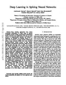
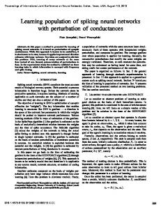
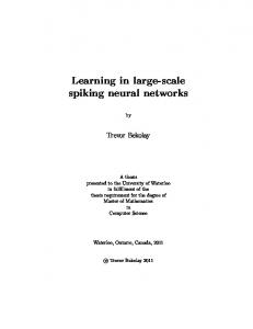
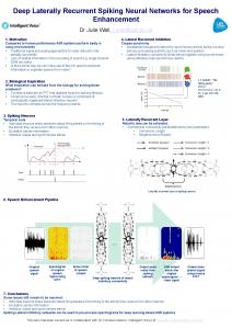
Such temporal translation can be achieved using networks of spiking neurons. Experimentation has shown that it is trivial to train an FFSNN with one input and one output to implement an arbitrary delay to high precision, so long as the desired delay does not exceed the temporal resolution at which the FFSNN operates. Thus multiple copies of these trained networks can be used to delay the firing times of recurrent units in parallel. Figure 1 shows a typical RSNN architecture used in our experiments. As in the general TIS (transformed input and state) memory model (Mozer, 1994), the network consists of five layers. Each input item is processed within a single simulation interval. The extended input layer (input and context layers, denoted by I and C, respectively) feeds the first auxiliary hidden layer H1 , which in turn feeds the recurrent layer Q. Within the n-th simulation interval, the spike timings of neurons in the input and context layers I and C are stored in the spatial spike train vectors i(n) and c(n), respectively. The spatial spike trains of the first hidden and recurrent layers are stored in vectors h1 (n) and q(n), respectively. The role of the recurrent layer Q is twofold: 1. The spike train q(n) codes information about the history of n inputs seen so far. This information is passed to the next simulation interval through the delay FFSNN network5 α, c(n + 1) = α(q(n)). The delayed spatial spike train c(n + 1) appears in the context layer. Spike train (i(n + 1), c(n + 1)) of the extended input in simulation interval n + 1, consists of the history-coding spike train c(n + 1) (representing the previously seen n inputs) and a spatial spike train i(n + 1) coding the current, (n + 1)-st, external input (input symbol) . 2. The recurrent layer feeds the second auxiliary hidden layer H2 , which finally feeds the output layer O. Within the n-th simulation interval, the spatial spike trains in the second hidden and output layers are stored in vectors h2 (n) and o(n), respectively. Parameters, such as the length Υ of the simulation interval, feedback delay ∆ and spike time encodings of input/output symbols have to be carefully coordinated. We illustrate this by unfolding an RSNN through two simulation periods (corresponding to processing of 2 input items) in Figure 2. The input string is ‘10‘ and the corresponding desired output string is ‘01‘. The input layer I has 5 neurons. There is a single neuron in the output layer O. All the other layers have 2 neurons each. Index n indexes the input items (and simulation intervals). Input symbols ’0’ and ’1’ are encoded in the five input units through spike patterns i0 = [0, 6, 0, 6, 0] and i1 = [0, 6, 6, 0, 0], respectively (all times are shown in ms). Spike patterns in the single output neuron for output symbols ’0’ and ’1’ are o0 = [20] and o1 = [26], respectively. Approximately 5ms elapses between the firing 5 the

delay function α(t) is applied to each component of q(n)

6

α

o(n)

O

h 2 (n)

H2

q(n)

Q

h1 (n)

H1

i(n)

I

Spike train o(n) encodes output for n−th input item

Spike train q(n) encodes state after presentation of n−th input item

delay by ∆

C

c(n) = α (q(n−1))

Spike train i(n) encodes n−th input item

Spike train c(n) is delayed state information from the previous input item presentation

Figure 1: Typical RSNN architecture used in our experiments. When processing the n-th input item, the external input is encoded through spike train i(n) in layer I, the state information is computed as spike train q(n) in layer Q and the output is represented by the spike train o(n) in layer O. Information about the inputs processed before seeing the n-th input item is contained in context spike train c(n) in layer C. c(n) = α(q(n − 1)) is state-encoding spike train from the previous time step, delayed by ∆. Hidden layers H1 and H2 (with spike trains h1 (n) and h2 (n), respectively) are auxiliary layers enhancing capabilities of the network to represent the state information and calculate the output.

7

n=1 t start (1) = 0ms

Target ’0’ coded as [20] t(1) = [20]

n=2 t start (2) = 40ms

o(1) = [22]

Target ’1’ coded as [26] t(2) = [66]

o(2) = [65]

h 2 (2) = [57,56]

h 2 (1) = [16,17]

q(1) = [12,11]

q(2) = [51,52]

α delay by ∆ = 30ms

h1 (1) = [7,8]

c(1) = c start

h 1 (2) = [48,47]

c(2) = [42,41]

i(1) = [0,6,6,0,0]

Input ’1’ coded as [0,6,6,0,0]

i(2)=[40,46,40,46,40]

Input ’0’ coded as [0,6,0,6,0]

Figure 2: The first two steps in the operation of an RSNN. The input string is ‘10‘ and the corresponding desired output is the string ‘01‘. The input layer I has 5 neurons. There is a single neuron in the output layer O. All the other layers have 2 neurons each. Spike train vectors are shown in ms. Processing of the n-th input symbol starts at tstart (n) = (n − 1) · 40ms. The target (desired) output patterns t(n) are shown above the output layers. Context spike train c(2) is the state spike train q(1) from the previous time step, delayed by ∆ = 30ms. The initial context spike train, cstart , is imposed externally at the beginning of training.

8

of neurons in each subsequent layer. Processing of the n-th input symbol starts at tstart (n) = (n − 1) · Υ,

(8)

where Υ = 40ms is length of the simulation interval. Spike train i(n) representing the n-th input symbol sn ∈ {0, 1} is calculated by shifting the corresponding input spike pattern isn by tstart (n), i(n) = isn + tstart (n). (9) The same principle applies to calculation of the target (desired) spike patterns t(n) that would be observed at the output, if the network functioned correctly. If, after presentation of the n-th input symbol sn , the desired output symbol is σn ∈ {0, 1}, then t(n) is calculated as t(n) = oσn + tstart (n). (10) The network is trained by minimizing the difference between the target and observed output spike patterns, t(n) and o(n), respectively. The training procedure is outlined in the next section. Context spike train c(2) is the state spike train q(1) from the previous time step, delayed by ∆ = 30ms. The initial context spike train, cstart , is imposed externally at the beginning of training.

3

Training – SpikePropThroughTime

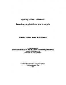
We extended the SpikeProp algorithm (Bohte, Kok & La Poutr´e, 2002) for training FFSNN to recurrent models in the spirit of Back Propagation Through Time for rate-based RNN (Werbos, 1989), i.e. using the unfolding-in-time methodology. We call this learning algorithm SpikePropThroughTime. Given an input string of length n, n copies of the base RSNN are made, stacked on top of each other, and sequentially simulated, incrementing tstart by Υ after each simulation interval. Expanding the base network through time via multiple copies simulates processing of the input stream by the base RSNN. Adaptation δ’s (see equations (4) and (6)) are calculated for each of the network copies. The synaptic efficacies (weights) in the base network are then updated using δ’s calculated in each of the copies by adding up, for every weight, the n corresponding weight-update contributions of equations (3) and (5). Figure 3 shows expansion through time of a five-layer base RSNN on an input of length 2. The first copy is simulated with tstart (1) = Υ · 0 = 0. As explained in the previous section, all firing times of the first copy are relative to 0. For copies n > 1, the external inputs and desired outputs are made relative to tstart (n) = (n − 1) · Υ. In a FFSNN, when calculating the δ’s for a hidden layer, the firing times from the preceding and succeeding layers are used. Special attention must be paid when calculating 9

o(2)

O

h2 (2)

Copy 2

H2

q(2)

h1 (2)

I

i(2)

o(1)

H1

c(2)

O

α

h2 (1)

H2

I

i(1)

C

Copy 1

delay by ∆

q(1)

h1 (1)

Q

Q

H1

c(1)

C

Figure 3: Expansion through time of a five-layer base RSNN on an input of length 2.

10

δ’s of neurons in the recurrent layer Q. Context spike train c(n + 1) in copy (n + 1) is the delayed recurrent spike train q(n) from the nth copy. The relationship of firing times in c(n + 1) and h1 (n + 1) contains the information that should be incorporated into the calculation of the δ’s for recurrent units in copy n. The delay constant ∆ is subtracted from the firing times h1 (n + 1) of H1 and then, when calculating the δ’s for recurrent units in copy n, these temporally translated firing times are used as if they were simply another hidden layer succeeding Q in copy n. Denoting by Γ2,n the set of neurons in the second auxiliary hidden layer H2 of the nth copy and by Γ1,n+1 the set of neurons in the first auxiliary hidden layer H1 of the copy (n + 1), the δ of the ith recurrent unit in the nth copy is calculated as

δ

= +

4

4.1

Pm

k k a a k a a k k=1 wij · ij (tj − ∆ − ti − dij ) · (1/(tj − ∆ − ti − dij ) − 1/τ )) Pm k k a a k a a k h∈Γi k=1 whi · hi (ti − th − dhi ) · (1/(ti − th − dhi ) − 1/τ ) P Pm k k a a k a a k j j∈Γ2,n ( k=1 wij · ij (tj − ti − dij ) · (1/(tj − ti − dij ) − 1/τ )) · δ P Pm k k a a k a a k h∈Γi k=1 whi · hi (ti − th − dhi ) · (1/(ti − th − dhi ) − 1/τ )

P i

j∈Γ1,n+1 (

· δj

P

(11)

Learning beyond finite memory in RSNN – inducing Moore machines Moore machines

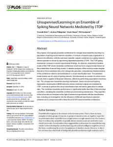
One of the simplest computational models that encapsulates the concept of unbounded input memory is the Moore machine (Hopcroft & Ullman, 1979). Formally, an (initial) Moore machine (MM) M is a 6-tuple M = (U, V, S, β, γ, s0 ), where U and V are finite input and output alphabets, respectively, S is a finite set of states, s0 ∈ S is the initial state, β : S ×U → S is the state transition function and γ : S → V is the output function. Given an input string u = u1 u2 ...un of symbols from U (ui ∈ U , i = 1, 2, ..., n), the machine M acts as a transducer by responding with the output string v = M (u) = v1 v2 ...vn , vi ∈ V , computed as follows: first the machine is initialized with the initial state s0 , then for all i = 1, 2, ..., n, the new state is recursively determined, si = β(si−1 , ui ), and the machine emits the output symbol vi = γ(si ). Moore machines are conveniently represented as directed labeled graphs: nodes represent states and arcs, labeled by symbols from U , represent state transitions initiated by the input symbols. An example of a simple MM is shown in figure 4

4.2

Encoding of input and output

In this study, we consider input alphabets of one, or two symbols. Moreover, there is a special end-of-string symbol ‘2’ initiating transitions to the initial state. In the experiments, 11

1

0

0 2

2

0

1

0

1

1

Figure 4: An example of a simple two-state Moore machine. Circles denote states. Arcs denote state transitions. The number in the upper-left of each state, labels it. The number in the lower-right of each state specifies its output value. Processing of each input string start in the initial state 0. Each arc is labeled with the input symbol initiating state transition specified by the arc. The special end-of-string reset symbol ‘2’ initiates a transition from every state to the initial state (dashed arcs). As an example: the input sequence 00111001 is mapped by the machine to the output sequence 00101110. the input layer I had five neurons. The input symbols ’0’, ’1’ and ’2’ are encoded in the five input units through spike patterns i0 = [0, 6, 0, 6, 0], i1 = [0, 6, 6, 0, 0] and i2 = [6, 0, 0, 6, 0], respectively. The firing times are in ms. The last input neuron acts like a reference neuron always firing at the beginning of any simulation interval. In all our experiments, we used binary output alphabet V = {0, 1} and the output layer O of RSNN consisted of a single neuron. Spike patterns (in ms) in the output neuron for output symbols ’0’ and ’1’ are o0 = [20] and o1 = [26], respectively.

4.3

Generation of training examples and learning

Given a target Moore machine M , a set of training examples is constructed by explicitly constructing input strings6 u over U and then determining the corresponding output string M (u) over V (by traversing edges of the graph of M , starting in the initial state, as prescribed by the input string u). The training set D consists of N couples of inputoutput strings, D = {(u1 , M (u1 )), (u2 , M (u2 )), ..., (uN , M (uN ))}. We adopt the strategy of inducing the initial state in the recurrent network (as opposed 6 It

is important to choose strings that exercise structures prominent in the target Moore machine, for example, if a Moore machine contains several discrete loops linked by transitions then the training string should exercise these loops and transitions. Random walks over the target machine, even those that exercise every transition, were found to be less effective at inducing structures than an intuitive exercising of the main structural components.

12

ˇ to externally imposing it – see (Forcada & Carrasco, 2005; Tiˇ no & Sajda, 1995)). The context layer of the network is initialized with the fixed predefined context spike train c(1) = cstart only at the beginning of training. From the network’s point of view, the training set is a couple (˜ u, M (˜ u)) of the long concatenated input sequence u ˜ = u1 2u2 2u3 2...2uN −1 2uN 2 and the corresponding output sequence M (˜ u) = M (u1 )γ(s0 )M (u2 )γ(s0 )M (u3 )γ(s0 )...γ(s0 )M (uN −1 )γ(s0 )M (uN )γ(s0 ). Input symbol ‘2’ is instrumental in inducing the start state by acting as an end-of-string reset symbol initiating transition from every state of M to the initial state s0 . The network is trained using SpikePropThroughTime (section 3) to minimize the squared error between the desired output spike trains derived from M (˜ u) when the RSNN is driven by the input u ˜. The RSNN is unfolded and SpikePropThroughTime is applied for each training pattern (ui , M (ui )), i = 1, 2, ..., N . In rate-based neural networks, the weights are conventionally initialized to random elements of < from the interval [0, 1]. For general feed forward networks of spiking neurons, it appears that this is not applicable when using the SpikeProp learning rule; learning of simple non-linear training sets appears to fail if the threshold is not sufficiently high, and the weights are not sufficiently scaled. The problem was first identified in (Moore, 2002)7 . The firing threshold is 50, and the weights are initialized to random elements of < from the interval8 (0, 10). We use a dynamic learning rate strategy that detects oscillatory behavior and plateaus within the error space. The action to take upon detecting oscillation or plateau, is respectively to decrease the learning rate by multiplying by an ‘oscillation-counter-coefficient’ (< 1), or increase the learning rate by multiplying by a ‘plateau-counter-coefficient’ (> 1) (see e.g. (Lawrence, Giles & Fong, 2000)).

4.4

Extraction of induced structure

It has been extensively verified in the context of traditional rate-based RNN that it is often possible to extract from RNN the target finite state machine M that the network 7 We

used the initial weight setting, neuron threshold parameters, and the learning rate as suggested by this thesis. 8 Whatever weight setting is chosen, the weights must be initialized so that the neurons in subsequent layers are sufficiently excited by those in their previous layer that they fire, otherwise the network would be unusable. There is no equivalent in traditional rate-based neural networks to the non-firing of a neuron in this sense. 13

was successfully trained and tested on. The extraction procedure operates on activation patterns appearing in the recurrent layer while processing9 M (e.g. (Giles et al., 1992; Tiˇ no ˇ & Sajda, 1995; Frasconi et al., 1996; Omlin & Giles, 1996); for an extensive review and criticism, see (Jacobsson, 2005)). One possibility10 is to drive the network with sufficiently long input strings and record the recurrent layer activations in a set B. The set B is then clustered using a vector-quantization tool. The cluster indexes will become states of the extracted finite state machine. Next, the network is first reset with repeated presentation of the the end-of-string symbol ‘2’ and then driven once more with sufficiently long input strings. At each time step n one records: • The index q˜(n) of the cluster containing the recurrent activation vector. The cluster index q˜(n) represents context cluster c˜(n + 1) = q˜(n) at time step n + 1. Given the current input symbol and context cluster c˜(n) = q˜(n − 1), the network transits (on the cluster level) to next context cluster c˜(n + 1) = q˜(n). • The network output associated with the next state11 c˜(n + 1) = q˜(n). Finally, the cluster transitions and output actions are summarized as a graph of a finite state machine that is minimized to its equivalent canonical form (Hopcroft & Ullman, 1979). The state information in RSNN is coded as spike trains in the recurrent layer Q. We studied whether, in analogy with rate-based RNN, the abstract information processing states can be discovered be detecting natural groupings of normalized spike trains12 (q(n)− tstart (n)) using a vector quantization tool (in our experiments – k-means clustering13 ). We also applied the extraction procedure to RSNN that managed to induce the target Moore machine only partially, so that the extent to which the target machine has been induced and the weaknesses of the induced mechanism can be exposed and understood. 9 with

frozen weights the Moore machine setting and RNN architecture used in this paper 11 If there are several output symbols associated with recurrent layer activations in the cluster q˜(n), the cluster q˜(n) is split so that the inconsistency is removed. 12 The spike times q(n) entering the quantization phase are made relative to the start time tstart (n) of the simulation interval 13 The goal here is to assign identical cluster indexes to ‘similar’ firing times and different indexes to ‘dissimilar’ firing times. Although the spiking neuron clustering method of (Natschl¨ager & Ruf, 1998) worked, k-means clustering is simpler (requires less hyperparameters) and faster, so was used in practice. 10 given

14

4.5

Experimental results

The network had 5 neurons in layers I, C, H1 , Q and H2 . Within each of those layers, one neuron was inhibitory, all the other ones were excitatory. Each connection between neurons had m = 16 synaptic channels, with delays dkij = k, k = 1, 2, ..., m, realizing axonal delays between 1ms and 16ms. The decay constant τ in response functions ij was set to τ = 3. The length Υ of the simulation interval was set to 40ms. The delay ∆ was 30ms. The inputs and desired outputs were coded into the spike trains as described in eqs. (8-10) and section 4.2. We used SpikePropThroughTime to train RSNN. The training was error-monitored and training was stopped when it was clear that the network had learned the target (zero thresholded output error) with sufficient stability. In some cases training was carried on until zero absolute error was achieved. The maximum number of training epochs (sweeps through the training set) was 10000. First, we experimented with ‘cyclic’ machines Cp of period p ≥ 2: U = {0}; V = {0, 1}; S = {0, 1, 2, ..., p − 1}; s0 = 0; for 0 ≤ i < p − 1, β(i, 0) = i + 1 and β(p − 1, 0) = 0; γ(0) = 0 and for 0 < i ≤ p − 1, γ(i) = 1. The RSNN perfectly learned machines Cp , 2 ≤ p < 5. After training, the respective RSNN emulated the operation of these MM perfectly and apparently indefinitely (no deviations from expected behavior were observed over test sets having length of the order 104 ). The training set had to be incrementally constructed by iteratively training with one presentation of the cycle, then two presentations etc. Note that given that the network can only observe the inputs, these MMs would require an unbounded input memory buffer. So no mechanism with vanishing (input) memory can implement string mappings represented by such MMs. Using the successful networks, we extracted unambiguously all the machines Cp of period 1 ≤ p < 5. The number of clusters in k-means clustering was set to 10. Second, we trained RSNN on a two-state machine M2 shown in figure 4. Again, the RSNN perfectly learned the machine14 . As in the previous experiment, no mechanism with vanishing input memory can implement string mappings defined by this Moore machine. Using the successful networks, we extracted unambiguously the machine M2 (the number of clusters in k-means clustering was 10). In the third experiment we investigate the information available in the context firing times in case of partial induction. Consider the three-state machine M3 in figure 5. The machine has two main fixed-input cycles in opposite directions. Training lead to an error ˜ 3 is rate of ≈ 0.3 over test strings of length 10000. The extracted induced machine M shown in figure 6. 14 Repeated

presentation of only 5 carefully selected training patterns of length 4 were sufficient for induction of this machine. No deviations from expected behavior were observed over test sets of length of the order 104 .

15

1

0

2

0

0

0 2

1

1 1

0

2

0

1

2 Figure 5: A three-state target Moore machine M3 that was partially induced.

2

2 2

0 0

1

2

0

1 2

1

4

0

1

0

3

0

1

0

0

1

0

1

0

1

1

5

1

2 2 ˜ 3 from a partial induction of the Moore machine M3 shown Figure 6: Extracted machine M in Figure 5.

16

The cycle on input ‘1’ in M3 has been successfully induced, but the cycle on input ‘0’ ˜ 3 corresponds with has not. The oscillation between states 4 and 1 on strings {01}+ in M the oscillation between states 1 and 2 in M3 . Transitions on the reset symbol ‘2’ have also ˜ 3 a cycle of length 4 (over the states 1,3,5,4) has been induced correctly. Curiously, in M been induced on fixed input ‘0’.

5

Discussion

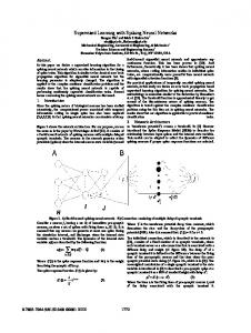
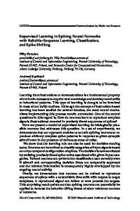
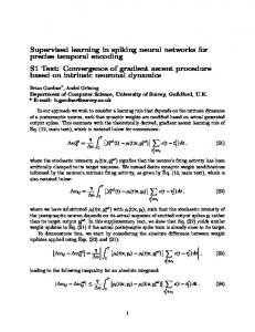
We were able to train RSNN to mimic target MMs requiring unbounded input memory on only a relatively simple set of MMs. Compared with traditional rate-based RNN, two major problems are apparent when inducing structures like MM in RSNN. 1. There are two timescales the network operates on: (i) the shorter timescale of spike trains coding the input, output and state information within a single simulation interval; and (ii) the longer timescale of sequences of simulation intervals, each representing a single input-to-output processing step. This time scale can be synchronized using spike oscillations as in (Natschl¨ager & Maass,2002). Long-term dynamics have to be induced based on the behavior of the target MM, but these dynamics are driven ultimately by the short-term dynamics of individual spikes. So in order to exhibit the desired long-term behavior, the network has to induce the appropriate short-term dynamics. In contrast, only the long-term dynamics need to be induced in the rate-base RNN. 2. Spiking neurons used in this paper produce a spike only when the accumulated potential xj (t) reaches a threshold Θ. This leads to discontinuities in the error-surface. Gradient-based methods for training feed-forward networks of spiking neurons alleviate this problem by resorting to simplifying assumptions on spike patterns within a single simulation interval (see (Bohte, Kok & La Poutr´e, 2002; Bohte, 2003)). The situation is much more complicated in the case of RSNN. A small weight perturbation can prevent a recurrent neuron from firing in the shorter time scale of a simulation interval. That in turn can have serious consequences for further longtime-scale processing. Especially so, if such a change in short-term behavior appears at the beginning of presentation of a long input string. The error surface becomes erratic, as evidenced in Figure 7. We took a RSNN trained to perfectly mimic the cycle-four machine C4 (see section 4.5). We studied the influence of perturbing weights w∗ in recurrent part of the RSNN (e.g. between layers I, C, H1 and Q) on the test error calculated on long test string of length 1000. For each weight perturbation extent ρ, we randomly sampled 100 weight vectors w from the hyperball of radius ρ centered at w∗ . Shown are the mean and standard 17

deviation values of the absolute output error per symbol for 0 < ρ ≤ 3. Clearly, small perturbations of weights lead to large abrupt changes in the test error. Obviously, gradient-based methods, like our SpikePropThroughTime have problems in locating good minima on such error surfaces. We tried • fast evolutionary strategies (FES) with (recommended) configuration (30,200)ES15 , employing the Cauchy mutation function (see (Yao & Liu, 1997; Yao, 1999)), • (extended) Kalman filtering in the parameter space (Puskorius & Feldkamp, 2002), and • a recent powerful evolutionary method for optimization on real-valued domains (Rowe & Hidovic, 2004) to find RSNN weights in the experiments in section 4.4, but without much success. The abrupt and erratic nature of the error surface makes it hard, even for evolutionary techniques, to locate a good minimum. We tried RSNNs with varying numbers of neurons in the hidden and recurrent layers. In general, the increased representational capacity of RSNNs with more neural units could not be utilized because of the problems with finding good weight settings due the erratic nature of the error surface. Our SpikePropThroughTime algorithm can be extended by allowing for adjustable axonal delays dkij , individual synaptic decay constants τijk and firing thresholds Θj (Schrauwen & Van Campenhout, 2004). While this may lead to models of reduced size, the inherent problems with learning instabilities will not be eliminated. We note that the finite memory machines induced in feed-forward spiking neuron networks (Natschl¨ager & Maass, 2002) (with dynamic synapses (Maass & Markram, 2002)) were quite simple (of depth 3). The input memory depth is limited by the feed-forward nature of such networks. As soon as one tries to increase processing capabilities of spiking networks by introducing feedback connections, while insisting on pulse-coding, the induction process becomes complicated. Theoretically, it is perfectly possible to emulate in a stable manner any MM in a sufficiently rich RSNN. For example, given a MM M , one needs to first fix appropriate spike patterns representing abstract states of the machine M . Then a FFSNN NS (playing the role of subnetwork of RSNN with layers C, I, H1 and Q) can be trained on the input driven state transition structure of M . The target spike trains on the top layer of NS are calculated by shifting the spike patterns representing states of M by an appropriate time delay ∆. Note that NS can be trained with traditional SpikeProp algorithm. While 15 in

each generation 30 parents generate 200 offspring through recombination and mu-

tation 18

Weight Perturbation vs Error for a Simple Four−State Automata

5

Standard Deviation Mean Over 100 Trials

4.5 4

Per Symbol Error

3.5 3 2.5 2 1.5 1 0.5 0

0

0.5

1

1.5 Absolute Perturbation Extent

2

2.5

3

Figure 7: Maximum radius of weight perturbation vs test error of RSNN trained to mimic the cycle-four machine C4 . For each setting of weight perturbation extent ρ, we randomly sampled 100 weight vectors w from the hyperball of radius ρ centered at induced RSNN weights w∗ . Shown are the mean (solid line) and standard deviation (dashed line) values of the absolute output error per symbol.

19

training, the target spike trains can be slightly perturbed to yield stable representations in NS of state transitions in M . Trained NS with added delay lines α (making spike trains at the top layer of NS appear in the context layer of NS with delay ∆) forms recurrent part of the RSNN being constructed. We need to stack another FFSNN NO on top of NS to associate states with outputs. Again, NO can be trained using SpikeProp to associate spike trains in top layer of NS (representing abstract states of M ) with the corresponding outputs. The target output spike trains need to be shifted by an appropriate simulation interval length Υ. Because processing in the spiking neuron networks is driven purely by relative differences between spike times in individual neurons, the RSNN consisting of NS (endowed with delay lines α) and NO will emulate M . Indeed, following this procedure we were able to construct a RSNN perfectly emulating e.g. machine M2 in figure 4 in a stable manner. Moreover, one can envisage a procedure for RSNN, analogous to that developed for rate-based RNN by Giles and Omlin (1993), that would enable direct insertion of (the whole, or part of) a given finite-state machine (FSM) into a RSNN. Such RSNN-based emulators of FSMs can be used as sub-modules in larger computational devices operating on spike trains. However, this paper aims to study induction of deeper-than-finite-input-memory temporal structures in RSNN. Finite state machines offer a convenient platform for our study, as they represent a simple, well established and easy to analyze framework for describing temporal structures that go beyond finite memory relationships. Many previous studies of inducing deep input memory structures in rate-based RNNs were performed in this frameˇ work (Cleeremans, Servan-Schreiber & McClelland, 1989; Giles et al., 1992; Tiˇ no & Sajda, 1995; Frasconi et al., 1996; Omlin & Giles, 1996; Casey, 1996; Tiˇ no et al., 1998). When training a RSNN on example string mappings drawn from some target MM, the structure of the target MM is assumed unknown for the learner. Hence, we cannot split training of RSNN into two separate phases (training two FFSNNs NS and NO on state transitions and state-output associations, respectively). RSNN is a dynamical system and weight changes in RSNN lead to complex bifurcation mechanisms, making it hard to induce more complex MM through a guided search in the weight space. It may be that in biological systems, long-term dependencies are represented using rate-based codings and/or a Liquid State Machine mechanism (Maass, Natschl¨ager & Markram, 2002) with a complex, but non-adaptable, recurrent pulse-coded part.

6

Conclusion

We have investigated possibilities of inducing temporal structures without fading memory in recurrent networks of spiking neurons operating strictly in the pulse-coding regime. All the input, output and state information is coded in terms of spike trains on subsets of

20

neurons. We briefly summarize key results of the paper. 1. A pulse-coding strategy for processing temporal information in recurrent spiking neuron networks (RSNN) was introduced. We have extended, in the sense of Back Propagation Through Time (Werbos, 1989), the gradient-based SpikeProp algorithm (Bohte, Kok & La Poutr´e, 2002) for training feed-forward spiking neuron networks (FFSNN). The algorithm, SpikePropThroughTime is able to account for temporal dependencies in the input stream when training RSNN. 2. We have shown that temporal structures with unbounded input memory specified by simple Moore machines can be induced by RSNN. The networks were able to discover pulse-coded representations of abstract information processing states coding potentially unbounded histories of processed inputs. However, the nature of pulsecoding, in the context of the training strategies tried here, appears not to allow induction beyond simple Moore machines. 3. In analogy with traditional rate-based RNN trained on finite state machines, it is often possible to extract from RSNN the target machines by grouping together similar spike trains appearing in the recurrent layer. Furthermore, extraction of finite-state machines from RSNN that managed to induce the target Moore machine only partially can reveal weaknesses of the induced mechanism and the extent to which the target machine has been learned. Even though, theoretically, RSNN operating on pulse coding can process any (computationally feasible) temporal structure of unbounded input memory, the induction of such structures through a guided search in the weight space is another matter. Weight changes in RSNN lead to complex bifurcation mechanisms, enormously complicating the training process.

References Abeles, M., Bergman, H., Gat I., Meilijson, I., Seidemann, E., Tishby, N., & Vaadia, E. (1995). Cortical activity flips among quasi stationary states. Proc. Natl. Acad. Sci. USA, 92, 8616–8620. Bengio, Y., Frasconi, P., & Simard, P. (1993). The problem of learning long-term dependencies in recurrent networks. In Proceedings of the 1993 IEEE International Conference on Neural Networks, Volume 3 (pp. 1183–1188).

21

Bohte, S., Kok, J., & La Poutr´e, H. (2002). Error-backpropagation in temporally encoded networks of spiking neurons. Neurocomputing, 48(1-4), 17–37. Bohte, S.M. (2003). Spiking Neural Networks. Ph.D. thesis, Centre for Mathematics and Computer Science (CWI), Amsterdam. Casey, M.P. (1996). The dynamics of discrete-time computation, with application to recurrent neural networks and finite state machine extraction. Neural Computation, 8(6), 1135–1178. Cleeremans, A., Servan-Schreiber, D, & McClelland, J.L. (1989). Finite state automata and simple recurrent networks. Neural Computation, 1(3), 372–381. DeWeese, M.R., & Zador, A.M. (2003). Binary coding in auditory cortex In S. Becker, S. Thrun, & K. Obermayer (Eds.), Advances in Neural Information Processing Systems 15 (pp. 101–108). MIT Press. Floreano, D., & Mattiussi, C. (2001). Evolution of spiking neural controllers for autonomous vision-based robots. In T. Gomi (Ed.), Evolutionary Robotics IV (pp. 38–61). LNCS, Springer–Verlag. Floreano, D., Zufferey, J., & Nicoud, J. (2005). From wheels to wings with evolutionary spiking neurons. Artificial Life, 11(1–2), 121–138. Forcada, M.L., & Carrasco, R.C. (1995). Learning the initial state of a second-order recurrent neural network during regular-language inference. Neural Computation, 7(5), 923–930. Frasconi, P., Gori, M., Maggini, M., & Soda, G. (1996). Insertion of finite state automata in recurrent radial basis function networks. Machine Learning, 23, 5–32. Gerstner, W. (1995). Time structure of activity in neural network models. Phys. Rev. E, 51, 738–758. Gerstner, W. (1999). Spiking neurons. In W. Maass, & C. Bishop (Eds.), Pulsed Coupled Neural Networks (pp. 3–54). Cambridge: MIT Press. Giles, C.L., Miller, C.B., Chen, D., Chen, H.H., Sun, G.Z., & Lee, Y.C. (1992). Learning and extracting finite state automata with second–order recurrent neural networks. Neural Computation, 4(3), 393–405. Giles, C.L., & Omlin, C.W. (1993). Insertion and Refinement of Production Rules in Recurrent Neural Networks. Connection Science, 5(3).

22

Hopcroft, J., & Ullman, J. (1979). Introduction to automata theory, languages, and computation. Reading, MA: Addison–Wesley. Jacobsson, H. (2005). Rule extraction from recurrent neural networks: A taxonomy and review. Neural Computation, 17(6), 1223 - 1263. Kn¨ usel, P., Wyss, R., K¨onig, P., & Verschure, P.F.M.J. (2004). Decoding a Temporal Population Code. Neural Computation, 16(10), 2079–2100. Lawrence, S., Giles, C.L., & Fong, S. (2000). Natural language grammatical inference with recurrent neural networks. IEEE Transactions on Knowledge and Data Engineering, 12(1), 126–140. Maass, W. (1996). Lower bounds for the computational power of networks of spiking neurons. Neural Computation, 8(1), 1–40. Maass, W., & Bishop, C. (Eds.) (2001). Pulsed Neural Networks. MIT Press. Maass, W., & Markram, H. (2002). Networks, 15(2), 155–161.

Synapses as dynamic memory buffers.

Neural

Maass, W., Natschl¨ager, T., & Markram, H. (2002). Real-time computing without stable states: A new framework for neural computation based on perturbations. Neural Computation, 14(11), 2531–2560. Martignon, L., Deco, G., Laskey, K.B., Diamond, M., Freiwald, W., & Vaadia, E. (2000). Neural coding: Higher-order temporal patterns in the neurostatistics of cell assemblies. Neural Computation, 12(11), 2621–2653. Moore, S. (2002). Back propagation in spiking neural networks (MSc thesis). The University of Bath, UK. Mozer, M.C. (1994). Neural net architectures for temporal sequence processing. In A. Weigend & N. Gershenfeld (Eds.), Predicting the future and understanding the past (pp. 243–264). Addison-Wesley Publishing. Nadasdy, Z., Hirase, H., Czurk, A., Csicsvari, J., & Buzski, G. (1999). Replay and time compression of recurring spike sequences in the hippocampus. The Journal of Neuroscience, 19(21), 9497–9507. Natschl¨ager, T., & Maass, W. (2002). Spiking neurons and the induction of finite state machines. Theoretical Computer Science: Special Issue on Natural Computing, 287(1), 251–265.

23

Natschl¨ager, T., & Ruf, B. (1998). Spatial and temporal pattern analysis via spiking neurons. Network: Computation in Neural Systems, 9(3), 319–332. Omlin, C., & Giles, C.L. (1996). Extraction of rules from discrete-time recurrent neural networks. Neural Networks, 9(1), 41–51. Puskorius, G., & Feldkamp, L. (1992). Recurrent network training with the decoupled extended Kalman filter. In Proceedings of the 1992 SPIE Conference on the Science of Artificial Neural Networks, Orlando, Florida. Rowe, J., & Hidovic, D. (2004). An evolution strategy using a continuous version of the gray-code neighbourhood distribution. In Proceedings of the Genetic and Evolutionary Computation Conference (GECCO-2004) (pp. 725–736). Lecture Notes in Computer Science, Springer-Verlag. Schrauwen, B., & Van Campenhout, J. (2004). Extending SpikeProp. In Proceedings of the International Joint Conference on Neural Networks, Budapest (pp. 471–476). Siegelmann, H., & Sontag, E. (1995). On the computational power of neural nets. Journal of Computer and System Sciences, 50(1), 132–150. Tiˇ no, P., Horne, B.G., Giles, C.L., & Collingwood, P.C. (1998). Finite state machines and recurrent neural networks – automata and dynamical systems approaches. In J.E. Dayhoff, & O. Omidvar (Eds.), Neural Networks and Pattern Recognition (pp. 171–220). Academic Press. ˇ Tiˇ no, P., & Sajda, J. (1995). Learning and extracting initial mealy machines with a modular neural network model. Neural Computation, 7(4), 822–844. Werbos, P. (1989). Generalization of backpropagation with applications to a recurrent gas market model. Neural Networks, 1(4), 339–356. Yao, X. (1999). Evolving artificial neural networks. Proceedings of the IEEE, 87(9), 1423–1447. Yao, X., & Liu, Y. (1997). Fast evolution strategies. Control and Cybernetics, 26(3), 467–496.

24