Learning Convex Combinations of Continuously Parameterized Basic

Learning Convex Combinations of Continuously Parameterized Basic Kernels Andreas Argyriou1 , Charles A. Micchelli2 , and Massimiliano Pontil1 1

2

Department of Computer Science, University College London, Gower Street, London WC1E 6BT, England, UK {a.argyriou, m.pontil}@cs.ucl.ac.uk Department of Mathematics and Statistics, State University of New York, The University at Albany, 1400 Washington Avenue, Albany, NY, 12222, USA

Abstract. We study the problem of learning a kernel which minimizes a regularization error functional such as that used in regularization networks or support vector machines. We consider this problem when the kernel is in the convex hull of basic kernels, for example, Gaussian kernels which are continuously parameterized by a compact set. We show that there always exists an optimal kernel which is the convex combination of at most m + 1 basic kernels, where m is the sample size, and provide a necessary and sufficient condition for a kernel to be optimal. The proof of our results is constructive and leads to a greedy algorithm for learning the kernel. We discuss the properties of this algorithm and present some preliminary numerical simulations.

1

Introduction

A common theme in machine learning is that a function can be learned from a finite set of input/output examples by minimizing a regularization functional which models a trade-off between an error term, measuring the fit to the data, and a smoothness term, measuring the function complexity. In this paper we focus on learning methods which, given examples {(xj , yj ) : j ∈ INm } ⊆ X × IR, estimate a real-valued function by minimizing the regularization functional q(yj , f (xj )) + µf 2K (1) Qµ (f, K) = j∈INm

where q : IR × IR → IR+ is a prescribed loss function, µ is a positive parameter and INm := {1, . . . , m}. The minimum is taken over f ∈ HK , a reproducing kernel Hilbert space (RKHS) with kernel K, see [1]. This approach has a long history. It has been studied, from different perspectives, in statistics [16], in optimal recovery [10], and more recently, has been

This work was supported by EPSRC Grant GR/T18707/01, NSF Grant ITR0312113 and the PASCAL European Network of Excellence.

P. Auer and R. Meir (Eds.): COLT 2005, LNAI 3559, pp. 338–352, 2005. c Springer-Verlag Berlin Heidelberg 2005

Learning Convex Combinations of Continuously Parameterized Basic Kernels

339

a focus of attention in machine learning theory, see, for example [14, 15] and references therein. The choice of the loss function q leads to different learning methods among which the most prominent have been square loss regularization and support vector machines. As new parametric families of kernels are being proposed to model functions defined on possibly complex/structured input domains (see, for example, [14] for a review) it is increasingly important to develop optimization methods for tuning kernel-based learning algorithms over a possibly large number of kernel parameters. This motivates us to study the problem of minimizing functional (1) not only over f but also over K, that is, we consider the variational problem Qµ (K) = inf{Qµ (f, K) : f ∈ HK , K ∈ K}

(2)

where K is a prescribed convex set of kernels. This point of view was proposed in [3, 8] where the problem (2) was mainly studied in the case of support vector machines and when K is formed by combinations of a finite number of basic kernels. Other related work on this topic appears in the papers [4, 9, 11, 18]. In this paper, we present a framework which allows us to model richer families of kernels parameterized by a compact set Ω, that is, we consider kernels of the type G(ω)dp(ω) : p ∈ P(Ω)

K=

(3)

Ω

where P(Ω) is the set of all probability measures on Ω. For example, when Ω ⊆ IR+ and the function G(ω) is a multivariate Gaussian kernel with variance ω then K is a subset of the class of radial kernels. The set-up for the family of kernels in (3) is discussed in Section 2, where we also review some earlier results from [9]. In particular, we establish that if q is convex then problem (2) is equivalent to solving a saddle-point problem. In Section 3, we derive optimality conditions for problem (2). We present a necessary and sufficient condition which characterizes a solution to this problem (see Theorem 2) and show that there ˆ with a finite representation. Specifically, for always exists an optimal kernel K this kernel the probability measure p in (3) is an atomic measure with at most m + 1 atoms (see Theorem 1). As we shall see, this implies, for example, that the optimal radial kernel is a finite mixture of Gaussian kernels when the variance is bounded above and away from zero. We mention, in passing, that a version of our characterization also holds when Ω is locally compact (see Theorem 4). The proof of our results is constructive and can be used to derive algorithms for learning the kernel. In Section 4, we propose a greedy algorithm for learning the kernel and present some preliminary experiments on optical character recognition.

2

Background and Notation

In this section we review our notation and present some background results from [9] concerning problem (2). We begin by recalling the notion of a kernel and RKHS HK . Let X be a set. By a kernel we mean a symmetric function K : X × X → IR such that for every

340

A. Argyriou, C.A. Micchelli, and M. Pontil

finite set of inputs x = {xj : j ∈ INm } ⊆ X and every m ∈ IN, the m × m matrix Kx := (K(xi , xj ) : i, j ∈ INm ) is positive semi-definite. We let L(IRm ) be the set of m × m positive semi-definite matrices and L+ (IRm ) the subset of positive definite ones. Also, we use A(X ) for the set of all kernels on the set X and A+ (X ) for the set of kernels K such that, for each m ∈ IN and each choice of x, Kx ∈ L+ (IRm ). According to Aronszajn and Moore [1], every kernel is associated with an (essentially) unique Hilbert space HK with inner product ·, ·K such that K is its reproducing kernel. This means that for every f ∈ HK and x ∈ X , f, Kx K = f (x), where Kx (·) := K(x, ·). Equivalently, any Hilbert space H of real-valued functions defined everywhere on X such that the point evaluation functionals Lx (f ) := f (x), f ∈ H are continuous on H, admits a reproducing kernel K. Let D := {(xj , yj ) : j ∈ INm } ⊆ X × IR be prescribed data and y the vector (yj : j ∈ INm ). For each f ∈ HK , we introduce the information operator Ix (f ) := (f (xj ) : j ∈ INm ) of values of f on the set x := {xj : j ∈ INm }. We let IR+ := [0, ∞), prescribe a nonnegative function Q : IRm → IR+ and introduce the regularization functional Qµ (f, K) := Q(Ix (f )) + µf 2K

(4)

:= f, f K and µ is a positive constant. Note that Q depends on where y but we suppress it in our notation as it is fixed throughout our discussion. For example, in equation (1) we have, for w = (wj : j ∈ Nn ), that Q(w) = j∈INm q(yj , wj ), where q is a loss function. Associated with the functional Qµ and the kernel K is the variational problem f 2K

Qµ (K) := inf{Qµ (f, K) : f ∈ HK }

(5)

which defines a functional Qµ : A(X ) → IR+ . We remark, in passing, that all of what we say about problem (5) applies to functions Q on IRm which are bounded from below as we can merely adjust the expression (4) by a constant independent of f and K. Note that if Q : IRm → IR+ is continuous and µ is a positive number then the infimum in (5) is achieved because the unit ball in HK is weakly compact. In particular, when Q is convex the minimum is unique since in this case the right hand side of equation (4) is a strictly convex functional of f ∈ HK . Moreover, if f is a solution to problem (5) then it has the form f (x) = cj K(xj , x), x ∈ X (6) j∈INm

for some real vector c = (cj : j ∈ INm ). This result is known as the Representer Theorem, see, for example, [14]. Although it is simple to prove, this result is remarkable as it makes the variational problem (5) amenable to computations. In particular, if Q is convex, the unique minimizer of problem (5) can be found by replacing f by the right hand side of equation (6) in equation (4) and then optimizing with respect to the vector c. That is, we have the finite dimensional variational problem Qµ (K) := min{Q(Kx c) + µ(c, Kx c) : c ∈ IRm }

(7)


341

where (·, ·) is the standard inner product on IRm . For example, when Q is the square loss defined for w = (wj : j ∈ INm ) ∈ IRm as Q(w) = w − y2 := 2 j∈INm (wj − yj ) the function in the right hand side of (7) is quadratic in the vector c and its minimizer is obtained by solving a linear system of equations. The point of view of this paper is that the functional (5) can be used as a design criterion to select the kernel K. To this end, we specify an arbitrary convex subset K of A(X ) and focus on the problem Qµ (K) := inf{Qµ (K) : K ∈ K}.

(8)

Every input set x and convex set K of kernels determines a convex set of matrices in L(IRm ), namely K(x) := {Kx : K ∈ K}. Obviously, it is this set of matrices that affects the variational problem (8). For this reason, we say that the set of kernels K is compact and convex provided that for all x the set of matrices K(x) is compact and convex. The following result is taken directly from [9]. Lemma 1. If K is a compact and convex subset of A+ (X ) and Q : IRm → IR is continuous then the minimum of (8) exists. The lemma requires that all kernels in K are in A+ (X ). If we wish to use kernels K only in A(X ) we may always modify them by adding any positive multiple of the delta function kernel ∆ defined, for x, t ∈ X , as 1, x = t ∆(x, t) = 0, x = t that is, replace K by K + a∆ where a is a positive constant. There are two useful cases of the set K of kernels which are compact and convex. The first is formed by the convex hull of a finite number of kernels in A+ (X ). The second case generalizes the above one to a compact Hausdorff space Ω (see, for example, [12]) and a mapping G : Ω → A+ (X ). For each ω ∈ Ω, the value of the kernel G(ω) at x, t ∈ X is denoted by G(ω)(x, t) and we assume that the function of ω → G(ω)(x, t) is continuous on Ω for each x, t ∈ X . When this is the case we say G is continuous. We let P(Ω) be the set of all probability measures on Ω and observe that G(ω)dp(ω) : p ∈ P(Ω) (9) K(G) := Ω

is a compact and convex set of kernels in A+ (X ). The compactness of this set is a consequence of the weak∗ -compactness of the unit ball in the dual space of C(Ω), the set of all continuous real-valued functions g on Ω with norm gΩ := max{|g(ω)| : ω ∈ Ω}, see [12]. For example, we choose Ω = [ω1 , ω2 ], where 2 0 < ω1 < ω2 and G(ω)(x, t) = e−ωx−t , x, t ∈ IRd , ω ∈ Ω, to obtain radial kernels, or G(ω)(x, t) = eω(x,t) to obtain dot product kernels. Note that the choice Ω = INn corresponds to the first case. Next, we establish that if the loss function Q : IRm → IR is convex then the functional Qµ : A+ (X ) → IR+ is convex as well, that is, the variational

342


problem (8) is a convex optimization problem. To this end, we recall that the conjugate function of Q, denoted by Q∗ : IRm → IR ∪ {+∞}, is defined, for every v ∈ IRm , as (10) Q∗ (v) = sup{(w, v) − Q(w) : w ∈ IRm } and it follows, for every w ∈ IRm , that Q(w) = sup{(w, v) − Q∗ (v) : v ∈ IRm }

(11)

see [5]. See also [17] for a nice application of the conjugate function to linear statistical models. For example, for the square loss defined above, the conjugate function is given, for every v ∈ IRm , by 1 Q∗ (v) = max (w, v) − w − y2 : w ∈ IRm = v2 + (y, v). 4 Note that Q∗ (0) = − inf{Q(w) : w ∈ IRm } < ∞ since Q is bounded from below. This observation is used in the proof of the lemma below. Lemma 2. If K ∈ A(X ), x is a set of m points of X such that Kx ∈ L+ (IRm ) and Q : IRm → IR a convex function then there holds the formula 1 (12) Qµ (K) = max − (v, Kx v) − Q∗ (v) : v ∈ IRm . 4µ The fact that the maximum above exists follows from the hypothesis that Kx ∈ L+ (IRm ) and the fact that Q∗ (v) ≥ −Q(0) for all v ∈ IRm , which follows from equation (10). The proof of the lemma is based on a version of the von Neumann minimax theorem (see the appendix). This lemma implies that the functional Qµ : A+ (X ) → IR+ is convex. Indeed, equation (12) expresses Qµ (K) as the maximum of linear functions in the kernel K.

3

Characterization of an Optimal Kernel

Our discussion in Section 2 establishes that problem (8) reduces to the minimax problem (13) Qµ (K) = − max{min{R(c, K) : c ∈ IRm } : K ∈ K} where the function R is defined as R(c, K) =

1 (c, Kx c) + Q∗ (c), 4µ

c ∈ IRm , K ∈ K.

(14)

In this section we show that problem (13) admits a saddle point, that is, the minimum and maximum in (13) can be interchanged and describe the properties of this saddle point. We consider this problem in the general case that K is induced by a continuous mapping G : Ω → A+ (X ) where Ω is a compact Hausdorff space, so we write K as K(G), see equation (9). We assume that the conjugate function is differentiable everywhere and denote the gradient of Q∗ at c by ∇Q∗ (c).


343

Theorem 1. If Ω is a compact Hausdorff topological space and G : Ω → A+ (X ) ˆ = is continuous then there exists a kernel K G(ω)dˆ p(ω) ∈ K(G) such that pˆ Ω is a discrete probability measure on Ω with at most m + 1 atoms and, for any atom ω ˆ ∈ Ω of pˆ, we have that R(ˆ c, G(ˆ ω )) = max{R(ˆ c, G(ω)) : ω ∈ Ω}

(15)

where cˆ is the unique solution to the equation 1 ˆ Kx cˆ + ∇Q∗ (ˆ c) = 0. 2µ

(16)

Moreover, for every c ∈ IRm and K ∈ K(G), we have that ˆ ≤ R(c, K). ˆ R(ˆ c, K) ≤ R(ˆ c, K)

(17)

Proof. Let us first comment on the nonlinear equation (16). For any kernel K ∈ K(G) the extremal problem min{R(c, K) : c ∈ IRm } has a unique solution, since the function c → R(c, K) is strictly convex and limc→∞ R(c, K) = ∞. Moreover, if we let cK ∈ IRm be the unique minimizer, it solves the equation 1 Kx cK + ∇Q∗ (cK ) = 0. 2µ Hence, equation (16) says that cˆ = cKˆ . ˆ described above. First, we Now let us turn to the existence of the kernel K note the immediate fact that max{R(c, K) : K ∈ K(G)} = max{R(c, G(ω)) : ω ∈ Ω}. Next, we define the function ϕ : IRm → IR by ϕ(c) := max{R(c, G(ω)) : ω ∈ Ω}, c ∈ IRm . According to the definition of the conjugate function in equation (10) and the hypotheses that G is continuous and {G(ω) : ω ∈ Ω} ⊆ A+ (X ) we see that limc→∞ ϕ(c) = ∞. Hence, ϕ has a minimum. We call a minimizer c˜. This vector is characterized by the fact that the right directional derivative of ϕ at c˜ c; d). in all directions d ∈ IRm is nonnegative. We denote this derivative by ϕ+ (˜ Using Lemma 4 in the appendix, we have that 1 ∗ ∗ (d, Gx (ω)˜ c; d) = max c) + (∇Q (˜ c), d) : ω ∈ Ω ϕ+ (˜ 2µ where the set Ω ∗ is defined as Ω ∗ := {ω : ω ∈ Ω, R(˜ c, G(ω)) = ϕ(˜ c)} .

344


1 If we define the vectors z(ω) = 2µ Gx (ω)˜ c + ∇Q∗ (˜ c), ω ∈ Ω ∗ , the condition that m c; d) is nonnegative for all d ∈ IR means that ϕ+ (˜

max{(z(ω), d) : ω ∈ Ω ∗ } ≥ 0,

d ∈ IRm .

Since G is continuous, the set N := {z(ω) : ω ∈ Ω ∗ } is a closed subset of IRm . Therefore, its convex hull M := co(N ) is closed as well. We claim that 0 ∈ M. Indeed, if 0 ∈ / M then there exists a hyperplane {c : c ∈ IRm , (w, c) + α = 0}, α ∈ IR, w ∈ IRm , which strictly separates 0 from M, that is, (w, 0) + α > 0 and (w, z(ω)) + α ≤ 0, ω ∈ Ω ∗ , see [12]. The first condition implies that α > 0 and, so we conclude that max{(w, z(ω)) : ω ∈ Ω ∗ } < 0 which contradicts our hypothesis that c˜ is a minimum of ϕ. By the Caratheodory theorem, see, for example, [5–Ch. 2], every vector in M can be expressed as a convex combination of at most m + 1 of the vectors in N . In particular, we have that 0= λj z(ωj ) (18) j∈INm+1 ∗ for some {ω j : j ∈ INm+1 } ⊆ Ω and nonnegative constants λj with j∈INm+1 λj = 1. Setting

ˆ := K

λj G(ωj ) =

j∈INm+1

G(ω)dˆ p(ω) Ω

where pˆ = j∈INm+1 λj δωj , (we denote by δω the Dirac measure at ω), we can rewrite equation (18) as 1 ˆ Kx c˜ + ∇Q∗ (˜ c) = 0. 2µ Hence, we conclude that c˜ = cˆ which means that ˆ : c ∈ IRm } = R(ˆ ˆ min{R(c, K) c, K). This establishes the upper inequality in (17). For the lower inequality we observe that ˆ R(ˆ c, G(ω))dˆ p(ω) = λj R(ˆ c, G(ωj )). R(ˆ c, K) = Ω

j∈INm+1

Since cˆ = c˜, we can use the definition of the ωj to conclude for any K ∈ K(G) by equation (18) and the definition of the function ϕ that ˆ = ϕ(ˆ R(ˆ c, K) c) ≥ R(ˆ c, K).

This theorem improves upon our earlier results in [9] where only the square ˆ of R loss function was studied in detail. Generally, not all saddle points (ˆ c, K)


345

satisfy the properties stated in Theorem 1. Indeed, a maximizing kernel may be ˆ = represented as K G(ω)dˆ p(ω) where pˆ may contain more than m + 1 atoms Ω or even have uncountable support (note, though, that the proof above provides a procedure for finding a kernel which is the convex combination of at most m + 1 kernels). With this caveat in mind, we show below that the conditions stated in Theorem 1 are necessary and sufficient. ˆ = G(ω)dˆ p(ω), where pˆ is a probability Theorem 2. Let cˆ ∈ IRm and K Ω ˆ ⊆ Ω. The pair (ˆ ˆ is a saddle point of problem (13) measure with support Ω c, K) ˆ satisfies equation (15). if and only if cˆ solves equation (16) and every ω ˆ∈Ω ˆ is a saddle point of (13) then cˆ is the unique minimizer of the Proof. If (ˆ c, K) ˆ and solves equation (16). Moreover, we have that function R(·, K) ˆ = max{R(ˆ R(ˆ c, G(ω))dˆ p(ω) = R(ˆ c, K) c, G(ω)) : ω ∈ Ω} ˆ Ω

ˆ implying that equation (15) holds true for every ω ˆ ∈ Ω. On the other hand, if cˆ solves equation (16) we obtain the upper inequality in equation (17) whereas equation (15) brings the lower inequality. Theorem 1 can be specified to the case that Ω is a finite set, that is K = co(Kn ) where Kn = {K : ∈ INn } is a prescribed set of kernels. Below, we use the notation Kx, for the matrix (K )x . ˆ = Corollary 1. If Kn = {Kj : j ∈ INn } ⊂ A+ (X ) there exists a kernel K λ K ∈ co(K ) such that the set J = {j : j ∈ IN , λ > 0} contains at n n j j∈INn j j most min(m + 1, n) elements and, for every j ∈ J we have that R(ˆ c, Kj ) = max{(R(ˆ c, K ) : ∈ INn }

(19)

where cˆ is the unique solution to the equation 1 ˆ Kx cˆ + ∇Q∗ (ˆ c) = 0. 2µ

(20)

Moreover, for every c ∈ IRm and K ∈ co(Kn ) we have that ˆ ≤ R(c, K). ˆ R(ˆ c, K) ≤ R(ˆ c, K)

(21)

In the important case that Ω = [ω1 , ω2 ] for 0 < ω1 < ω2 and G(ω) is a Gaussian kernel, G(ω)(x, t) = exp(−ωx−t2 ), x, t ∈ IRd , Theorem 1 establishes that a mixture of at most m + 1 Gaussian kernels provides an optimal kernel. What happens if we consider all possible Gaussians, that is, take Ω = IR+ ? This question is important because Gaussians generate the whole class of radial kernels. Indeed, we recall a beautiful result by I.J. Schoenberg [13]. Theorem 3. Let h be a real-valued function defined on IR+ such that h(0) = 1. We form a kernel K on IRd × IRd by setting, for each x, t ∈ IRd , K(x, t) =

346


h(x − t2 ). Then K is positive definite for any d if and only if there is a probability measure p on IR+ such that 2 e−ωx−t dp(ω), x, t ∈ IRd . K(x, t) = IR+

Note that the set IR+ is not compact and the kernel G(0) is not in A+ (IRd ). Therefore, on both accounts Theorem 1 does not apply in this circumstance. In general, we may overcome this difficulty by a limiting process which can handle kernel maps on locally compact Hausdorff spaces. This will lead us to an extension of Theorem 1 where Ω is locally compact. However, we only describe our approach in detail for the Gaussian case and Ω = IR+ . An important ingredient in the discussion presented below is that G(∞) = ∆, the diagonal kernel. Furthermore, in the statement of the theorem below it is understood that when we say that pˆ is a discrete probability measure on IR+ we mean that pˆ can have an atom not only at zero but also at infinity. Therefore, we can integrate any function relative to such a discrete measure over the extended positive real line provided such a function is defined therein. Theorem 4. Let G : IR+ → A(X ) be defined as 2

G(ω)(x, t) = e−ωx−t , x, t ∈ IRd , ω ∈ IR+ . ˆ = Then there exists a kernel K G(ω)dˆ p(ω) ∈ K(G) such that pˆ is a discrete IR+ ˆ ∈ IR+ probability measure on IR+ with at most m + 1 atoms and, for any atom ω of pˆ, we have that R(ˆ c, G(ˆ ω )) = max{R(ˆ c, G(ω)) : ω ∈ IR+ }

(22)

where cˆ is a solution to the equation 1 ˆ Kx cˆ + ∇Q∗ (ˆ c) = 0 2µ

(23)

and the function Q∗ is continuously differentiable. Moreover, for every c ∈ IRm and K ∈ K(G), we have that ˆ ≤ R(c, K). ˆ R(ˆ c, K) ≤ R(ˆ c, K)

(24)

Proof. For every ∈ IN we consider the Gaussian kernel map on the interval −1 ˆ = Theorem 1 to produce a sequence of kernels K Ω := [ , ] and appeal to m G(ω)dˆ p (ω) and c ˆ ∈ IR with the properties described there. In particular, pˆ Ω is a discrete probability measure with at most m+1 atoms, a number independent of . Let us examine what may happen as tends towards infinity. Each of the atoms of pˆ as well as their corresponding weights have subsequences which converge. Some atoms may converge to zero while others to infinity. In either case, the Gaussian kernel map approaches a limit. Therefore, we can extract a


347

ˆn : convergent subsequence {ˆ pn : ∈ IN} of probability measures andkernels {K ˆ n = K, ˆ and K ˆ = G(ω)dˆ p(ω) ∈ IN} such that lim→∞ pˆn = pˆ, lim→∞ K IR+ with the provision that pˆ may have atoms at either zero or infinity. In either case, we replace the Gaussian by its limit, namely G(0), the identically one kernel, or ˆ G(∞), the delta kernel, in the integral which defines K. ˆ To establish that K is an optimal kernel, we turn our attention to the sequence of vectors cˆn . We claim that this sequence also has a convergent subsequence. Indeed, from equation (17) for every K = Ω G(ω)dp(ω), p ∈ P(Ω ) we have that ˆ n ) = Q∗ (0) < ∞. R(ˆ cn , K) ≤ R(0, K Using the fact that the function Q∗ is bounded below (see our comments after the proof of Lemma 2) we see that the sequence cˆn has Euclidean norm bounded independently of . Hence, it has a convergent subsequence whose limit we call cˆ. Passing to the limit we obtain equations (23) and (24) and, so, conclude that ˆ is a saddle point. (ˆ c, K) We remark that extensions of the results in this section also hold true for nondifferentiable convex functions Q. The proofs presented above must be modified in this general case in detail but not in substance. We postpone the discussion of this issue to a future occasion.

4

A Greedy Algorithm for Learning the Kernel

The analysis in the previous section establishes necessary and sufficient condiˆ ∈ IRm × K(G) to be a saddle point of the problem tions for a pair (ˆ c, K) −Qµ (G) := max {min {R(c, K) : c ∈ IRm } : K ∈ K(G)} . ˆ Indeed, once The main step in this problem is to compute the optimal kernel K. ˆ K has been computed, cˆ is obtained as the unique solution cK to the equation 1 Kx cK + ∇Q∗ (cK ) = 0 2µ

(25)

ˆ for K = K. With this observation in mind, in this section we focus on the computational issues for the problem − Qµ (G) = max{g(K) : K ∈ K(G)}

(26)

where the function g : A+ (X ) → IR is defined as g(K) := min {R(c, K) : c ∈ IRm } ,

K ∈ A+ (X ).

(27)

We present a greedy algorithm for learning an optimal kernel. The algorithm starts with an initial kernel K (1) ∈ K(G) and computes iteratively a sequence of kernels K (t) ∈ K(G) such that g(K (1) ) < g(K (2) ) < · · · < g(K (s) )

(28)

348

A. Argyriou, C.A. Micchelli, and M. Pontil Initialization: Choose K (1) ∈ K(G) For t = 1 to T : 1. Compute c(t) = argmin{R(c, K (t) ) : c ∈ IRm } using equation (25) (t)

2. Find ω ˆ ∈ Ω : (c(t) , Gx (ˆ ω )c(t) ) > (c(t) , Kx c(t) ). If such ω ˆ does not exist terminate ˆ = argmax{g(λG(ˆ 3. Compute λ ω ) + (1 − λ)K (t) ) : λ ∈ (0, 1]} ˆ ω ) + (1 − λ)K ˆ (t) 4. Set K (t+1) = λG(ˆ Fig. 1. Algorithm to compute an optimal convex combination of kernels in the set {G(ω) : ω ∈ Ω}

where s is the number of iterations. At each iteration t, 1 ≤ t ≤ s, the algorithm searches for a value ω ˆ ∈ Ω, if any, such that (c(t) , Gx (ˆ ω )c(t) ) > (c(t) , Kx(t) c(t) ) (t)

(29) (t+1)

where we have defined c := cK (t) . If such ω ˆ is found then a new kernel K is computed to be the optimal convex combination of the kernels G(ˆ ω ) and K (t) , that is,

ω ) + (1 − λ)K (t) ) : λ ∈ [0, 1] . (30) g(K (t+1) ) = max g(λG(ˆ If no ω ˆ ∈ Ω satisfying inequality (29) can be found, the algorithm terminates. The algorithm is summarized in Figure 1. Step 2 of the algorithm is implemented with a local gradient ascent in Ω. If the value of ω found locally does not satisfy inequality (29), the smallest hyperrectangle containing the search path is removed and a new local search is started in the yet unsearched part of Ω, continuing in this way until either the whole of Ω is covered or inequality (29) is satisfied. Although in the experiments below we will apply this strategy when Ω is an interval, it also naturally applies to more complex parameter spaces, for example a compact set in a Euclidean space. Step 3 is a simple maximization problem which we solve using Newton method, since the function g(λG(ˆ ω ) + (1 − λ)K (t) ) is concave in λ and its derivative can be computed by applying Lemma 4. We also use a tolerance parameter to enforce a non-zero gap in inequality (29). A version of this algorithm for the case when Ω = INn has also been implemented (below, we refer to this version as the “finite algorithm”). It only differs from the continuous version in Step 2, in that inequality (29) is tested by trial and error on randomly selected kernels from Kn . We now show that after each iteration, either the objective function g increases or the algorithm terminates, that is, inequality (28) holds true. To this end, we state the following lemma whose proof follows immediately from Theorem 2. Lemma 3. Let K1 , K2 ∈ A+ (X ). Then, λ = 0 is not a solution to the problem max {g(λK1 + (1 − λ)K2 ) : λ ∈ [0, 1]} if and only if R(cK2 , K1 ) > R(cK2 , K2 ).


349

Applying this lemma to the case that K1 = G(ˆ ω ) and K2 = K (t) we conclude that g(K (t+1) ) > g(K (t) ) if and only if ω ˆ satisfies the inequality R(c(t) , G(ˆ ω )) > R(c(t) , K (t) ) which is equivalent to inequality (29). 4.1

Experimental Validation

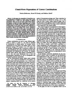
We have tested the above algorithm on eight handwritten digit recognition tasks of varying difficulty from the MNIST data-set1 . The data are 28×28 images with pixel values ranging between 0 and 255. We used Gaussian kernels as the basic kernels, that is, G(σ)(x, t) = exp(−x − t2 /σ 2 ), σ ∈ [σ1 , σ2 ]. In all the experiments, the test error rates were measured over 1000 points from the MNIST test set. The continuous and finite algorithms were trained using the square loss and compared to an SVM2 . In all experiments, the training set consisted of 500 points. For the finite case, we chose ten Gaussian kernels with σ’s equally spaced in an interval [σ1 , σ2 ]. For both versions of our algorithm, the starting value of the kernel was the average of these ten kernels and the regularization parameter was set to 10−7 . This value typically provided the best test performance among the nine values µ = 10− , ∈ {3, . . . , 11}. The performance of the SVM was obtained as the best among the results for the above ten kernels and nine values of µ. This strategy slightly favors the SVM but compensates for the fact that the loss functions are different. The parameters and T of our algorithm were chosen to be 10−3 and 100 respectively. Table 1 shows the results obtained. The range of σ is [75, 25000] in columns 2–4, [100, 10000] in columns 5–7 and [500, 5000] in columns 8–10. Note that, in most cases, the continuous algorithm finds a better combination of kernels than the finite version. In general, the continuous algorithm performs better than the SVM, whereas most of the time the finite algorithm is worse than the SVM. Moreover, the results indicate that the continuous algorithm is not affected by the range of σ, unlike the other two methods. Typically, the continuous algorithm requires less than 20 iterations to terminate whereas the finite algorithm may require as much as 100 iterations. Figure 2 depicts the convergence behavior of the continuous algorithm on two different tasks. In both cases σ ∈ [100, 10000]. The actual values of Qµ are six orders of magnitude smaller, but they were rescaled to fit the plot. Note that, in agreement with inequality (28), Qµ decreases and eventually converges. The misclassification error also converges to a lower value, indicating that Qµ provides a good learning criterion. 1 2

Available at: http://yann.lecun.com/exdb/mnist/index.html Trained using SVM-light, see: http://www.cs.cornell.edu/People/tj/svm light

350


Table 1. Misclassification error percentage for the continuous and finite versions of the algorithm and the SVM on different handwritten digit recognition tasks. See text for description Task \ Method Cont. Finite SVM σ ∈ [75, 25000] odd vs. even 6.6 18.0 11.8 3 vs. 8 3.8 6.9 6.0 4 vs. 7 2.5 4.2 2.8 1 vs. 7 1.8 3.9 1.8 2 vs. 3 1.6 3.9 3.1 0 vs. 6 1.6 2.2 1.7 2 vs. 9 1.5 3.2 1.9 0 vs. 9 0.9 1.2 1.1

Cont. Finite SVM σ ∈ [100, 10000] 6.6 10.9 8.6 3.8 4.9 5.1 2.5 2.7 2.6 1.8 1.8 1.8 1.6 2.8 2.3 1.6 1.7 1.5 1.5 1.9 1.8 0.9 1.0 1.0

Cont. Finite SVM σ ∈ [500, 5000] 6.5 6.7 6.9 3.8 3.7 3.8 2.5 2.6 2.3 1.8 1.9 1.8 1.6 1.7 1.6 1.6 1.6 1.5 1.5 1.4 1.4 0.9 0.9 1.0

0.065

0.072

0.06 0.07

0.055 0.05

0.068

0.045 0.066

0.04 0.035

0.064

0.03 0.062

5

10

15

20

0.025 1

2

3

4

5

6

7

Fig. 2. Functional Qµ (solid line) and misclassification error (dotted line) after the first iteration of the algorithm of Figure 1 for even vs. odd (left) and 3 vs. 8 (right)

5

Conclusion

We have studied the problem of learning a kernel which minimizes a convex error functional over the convex hull of prescribed basic kernels. The main contribution of this paper is a general analysis of this problem when the basic kernels are continuously parameterized by a compact set. In particular, we have shown that there always exists an optimal kernel which is a finite combination of the basic kernels and presented a greedy algorithm for learning a suboptimal kernel. The algorithm is simple to use and our preliminary findings indicate that it typically converges in a small number of iterations to a kernel with a competitive statistical performance. In the future we shall investigate the convergence properties of the algorithm, compare it experimentally to previous related methods for learning the kernel, such as those in [3, 6, 8], and study generalization error bounds for this problem. For the latter purpose, the results in [4, 18] may be useful.


351

References 1. N. Aronszajn. Theory of reproducing kernels. Trans. Amer. Math. Soc., 686, pp. 337–404, 1950. 2. J.P. Aubin. Mathematical Methods of Game and Economic Theory. Studies in Mathematics and its applications, Vol. 7, North-Holland, 1982. 3. F.R. Bach, G.R.G Lanckriet and M.I. Jordan. Multiple kernels learning, conic duality, and the SMO algorithm. Proc. of the Int. Conf. on Machine Learning, 2004. 4. O. Bousquet and D.J.L. Herrmann. On the complexity of learning the kernel matrix. Advances in Neural Information Processing Systems, 15, 2003. 5. J.M. Borwein and A.S. Lewis. Convex Analysis and Nonlinear Optimization. Theory and Examples. CMS (Canadian Math. Soc.) Springer-Verlag, New York, 2000. 6. O. Chapelle, V.N. Vapnik, O. Bousquet and S. Mukherjee. Choosing multiple parameters for support vector machines. Machine Learning, 46(1), pp. 131–159, 2002. 7. M. Herbster. Relative Loss Bounds and Polynomial-time Predictions for the KLMS-NET Algorithm. Proc. of the 15-th Int. Conference on Algorithmic Learning Theory, October 2004. 8. G.R.G. Lanckriet, N. Cristianini, P. Bartlett, L. El Ghaoui and M.I. Jordan. Learning the kernel matrix with semi-definite programming. J. of Machine Learning Research, 5, pp. 27–72, 2004. 9. C.A. Micchelli and M. Pontil. Learning the kernel function via regularization. To appear in J. of Machine Learning Research (see also Research Note RN/04/11, Department of Computer Science, UCL, June 2004).. 10. C. A. Micchelli and T. J. Rivlin. Lectures on optimal recovery. In Lecture Notes in Mathematics, Vol. 1129, P. R. Turner (Ed.), Springer Verlag, 1985. 11. C.S. Ong, A.J. Smola, and R.C. Williamson. Hyperkernels. Advances in Neural Information Processing Systems, 15, S. Becker, S. Thrun, K. Obermayer (Eds.), MIT Press, Cambridge, MA, 2003. 12. H.L. Royden. Real Analysis. Macmillan Publ. Company, New York, 3rd ed., 1988. 13. I.J. Schoenberg. Metric spaces and completely monotone functions. Annals of Mathematics, 39, pp. 811–841, 1938. 14. J. Shawe-Taylor and N. Cristianini. Kernel Methods for Pattern Analysis. Cambridge University Press, 2004. 15. V.N. Vapnik. Statistical Learning Theory. Wiley, New York, 1998. 16. G. Wahba. Spline Models for Observational Data. Series in Applied Mathematics, Vol. 59, SIAM, Philadelphia, 1990. 17. T. Zhang. On the dual formulation of regularized linear systems with convex risks. Machine Learning, 46, pp. 91–129, 2002. 18. Q. Wu, Y. Ying and D.X. Zhou. Multi-kernel regularization classifiers. Preprint, City University of Hong Kong, 2004.

A

Appendix

The first result we record here is a useful version of the classical von Neumann minimax theorem we have learned from [2–Ch. 7].

352


Theorem 5. Let h : A × B → IR where A is a closed convex subset of a Hausdorff topological vector space X and B is a convex subset of a vector space Y. If the function x → h(x, y) is convex and lower semi-continuous for every y ∈ B, the function y → h(x, y) is concave for every x ∈ A and there exists a y0 ∈ B such that for all λ ∈ IR the set {x : x ∈ A, h(x, y0 ) ≤ λ} is compact then there is an x0 ∈ A such that sup{h(x0 , y) : y ∈ B} = sup{inf{h(x, y) : x ∈ A} : y ∈ B}. In particular, we have that min{sup{h(x, y) : y ∈ B} : x ∈ A} = sup{inf{h(x, y) : x ∈ A} : y ∈ B}.

(31)

The hypothesis of lower semi-continuity means, for all λ ∈ IR and y ∈ B, that the set {x : x ∈ A, h(x, y) ≤ λ} is a closed subset of A. The next result concerns differentiation of a “max” function. Its proof can be found in [9]. Lemma 4. Let X be a topological vector space, T a compact set and G(t, x) a real-valued function on T × X such that, for every x ∈ X G(·, x) is continuous on T and, for every t ∈ T , G(t, ·) is convex on X . We define the real-valued convex function g on X as g(x) := max{G(t, x) : t ∈ T }, x ∈ X and the set M (x) := {t : t ∈ T , G(t, x) = g(x)}. Then the right derivative of g in the direction y ∈ X is given by g+ (x, y) = max{G+ (t, x, y) : t ∈ M (x)}

where G+ (t, x, y) is the right derivative of G with respect to its second argument in the direction y. Proof of Lemma 2. Theorem 5 applies since Kx ∈ L+ (IRm ). Indeed, we let h(c, v) = (Kx c, v) − Q∗ (v) + µ(c, Kx c), A = IRm , B = {v : Q∗ (v) < ∞, v ∈ IRm } and v0 = 0. Then, B is convex and, for any λ ∈ IR, the set {c : c ∈ IRm , h(c, v0 ) ≤ λ} is compact. Therefore, all the hypotheses of Theorem 5 hold. Consequently, using (11) in (7) we have that Qµ (K) = sup{min{(Kx c, v) − Q∗ (v) + µ(c, Kx c) : c ∈ IRm } : v ∈ B}.

(32)

For each v ∈ B, the minimum over c satisfies the equation Kx v + 2µKx c = 0, implying that min{(Kx c, v) − Q∗ (v) + µ(c, Kx c) : c ∈ IRm } = − and the result follows.

(v, Kx v) − Q∗ (v) 4µ