plete and noisy ICA [1]. Furthermore, favorable properties of sparse codes with respect to noise resistance have been studied [2]. Mathematically the problem.
ESANN'2008 proceedings, European Symposium on Artificial Neural Networks - Advances in Computational Intelligence and Learning Bruges (Belgium), 23-25 April 2008, d-side publi., ISBN 2-930307-08-0.
Learning Data Representations with Sparse Coding Neural Gas Kai Labusch and Erhardt Barth and Thomas Martinetz University of L¨ ubeck - Institute for Neuro- and Bioinformatics Ratzeburger Alle 160 23538 L¨ ubeck - Germany Abstract. We consider the problem of learning an unknown (overcomplete) basis from an unknown sparse linear combination. Introducing the “sparse coding neural gas” algorithm, we show how to employ a combination of the original neural gas algorithm and Oja’s rule in order to learn a simple sparse code that represents each training sample by a multiple of one basis vector. We generalise this algorithm using orthogonal matching pursuit in order to learn a sparse code where each training sample is represented by a linear combination of k basis elements. We show that this method can be used to learn artificial sparse overcomplete codes.
1
Introduction
In the last years there has been a lot of interest in sparse coding. Sparse coding is closely connected to independent component analysis, in particular to overcomplete and noisy ICA [1]. Furthermore, favorable properties of sparse codes with respect to noise resistance have been studied [2]. Mathematically the problem is to estimate an overcomplete basis of given training samples X = (x1 , . . . , xL ), xi ∈ ℜN that were generated from a sparse linear combination. Without loss of generality we require X to have zero mean. We measure the quality of the basis by the mean square of the representation error: L
E=
1X kxi − Ca(i)k22 L i=1
(1)
C = (c1 , . . . , cM ), cj ∈ ℜN denotes a matrix containing the basis elements. a(i) denotes a set of sparse coefficients that was chosen optimally for given xi and C. The number of basis elements M is a free model parameter. In case of overcomplete bases M > N holds. Imposing different constraints on the basis C or the choice of the coefficients a(i) allows to control the structure of the learned basis.
2
Vector quantization
A well-known approach for data representation is vector quantization. Vector quantization is based on a set of so-called codebook vectors. Each sample is encoded by the closest codebook vector. Therefore, for the coefficients a(i) holds (2) a(i)k = 1, a(i)j = 0 ∀j 6= k where k = arg minkcj − xi k22 j
233
ESANN'2008 proceedings, European Symposium on Artificial Neural Networks - Advances in Computational Intelligence and Learning Bruges (Belgium), 23-25 April 2008, d-side publi., ISBN 2-930307-08-0.
Vector quantization finds a set of codebook vectors that minimize (1) under the constraints posed by (2). The well-known k-means algorithm is among the methods that try to solve this optimization problem. But k-means can lead to a sub-optimal utilization of the codebook vectors with respect to (1) due to the hard-competitive nature of its learning scheme. The neural gas algorithm introduced in [3] remedies this deficiency by using a soft-competitive learning scheme that facilitates an optimal distribution of the codebook vectors over the data manifold to be learned.
3
Learning one-dimensional representations
In a step towards a more flexible coding scheme, i.e., a coding scheme that in some cases may better resemble the structure of the data, we drop one constraint on the coefficients a(i) allowing a representation in terms of an arbitrary multiple of one codebook vector. Due to the added flexibility of the coefficients, we require kcj k22 = 1 without loss of generality. This leads to the following optimization problem, which can be understood as a model of maximum sparseness: min
L X
kxi − Ca(i)k22
subject to
ka(i)k0 ≤ 1 and kcj k22 = 1
(3)
i
Here ka(i)k0 denotes the number of non-zero coefficients in a(i). First consider the marginal case of (3), where only one codebook vector is available, i.e, M = 1. Now (3) becomes: min
L X
kxi − ca(i)k22 =
i=1
L X
xTi xi − 2a(i)cT xi + a(i)2 subject to kck22 = 1 (4)
i=1
Fixing xi and c, (4) becomes minimal by choosing a(i) = cT xi . One obtains as final optimization problem: max
L X
(cT xi )2
subject to
kck22 = 1
(5)
i=1
Hence, in this marginal case, the problem of finding the codebook vector that minimizes (4) boils down to finding the direction of maximum variance. A wellknown learning rule that solves (5), i.e., that finds the direction of maximum variance, is called Oja’s rule [4]. Now we describe how to modify the original neural gas algorithm (see Algorithm 1) to solve the general case of (3), where M > 1 holds. The soft-competitive learning is achieved by controlling the update of all codebook vectors by the relative distances between the codebook vectors and the winning codebook vector. These distances are computed within the sample space (see Algorithm 1, step 4,5). Replacing the distance measure, we now consider the following sequence of distances: �2 �2 �2 − cTj0 x ≤ · · · ≤ − cTjk x ≤ · · · ≤ − cTjM x (6)
234
ESANN'2008 proceedings, European Symposium on Artificial Neural Networks - Advances in Computational Intelligence and Learning Bruges (Belgium), 23-25 April 2008, d-side publi., ISBN 2-930307-08-0.
Algorithm 1 The neural gas algorithm 1 initialize C = (c1 , . . . , cM ) using uniform random values for t = 0 to tmax do 2 select random sample x out of X 3 calculate current size of neighbourhood and learning rate: ` ´t/tmax λt = λ0 λf inal /λ0 ` ´t/tmax ǫt = ǫ0 ǫf inal /ǫ0 4
determine the sequence j0 , . . . , jM with: kx − cj0 k ≤ · · · ≤ kx − cjk k ≤ · · · ≤ kx − cjM k
5
for k = 1 to M do ` ´ update cjk according to cjk = cjk + ǫt e−k/λt cjk − x end for end for
Due to the modified distance measure a new update rule is required to minimize the distances between the codebook vectors and the current training sample x. According to Oja’s rule, with y = cTjk x, we obtain: cjk = cjk + ǫt e−k/λt y (x − ycjk )
(7)
Due to the optimization constraint kcj k = 1, we normalize the codebook vectors in each learning step. The complete “sparse coding neural gas” algorithm is shown in Algorithm 2.
4
Learning sparse codes with k-coefficients
In order to generalise the “Sparse Coding Neural Gas” algorithm, i.e., allowing for a representation using a linear combination of k elements of C to represent a given sample xi , we consider the following optimization problem: min
L X
kxi − Ca(i)k22 subject to ka(i)k0 ≤ k and kcj k22 = 1
(8)
i
A number of approximation methods tackling the problem of finding optimal coefficients a(i) constrained by ka(i)k0 ≤ k given fixed C and xi were proposed. It can be shown that in well-behaved cases methods such as matching pursuit or orthogonal matching pursuit [5] provide an acceptable approximation [6, 2]. We generalize the “sparse coding neural gas” algorithm with respect to (8) by performing in each iteration of the algorithm k steps of orthogonal matching pursuit. Given a sample x that was chosen randomly out of X, we initialize U = ∅, xres = x and R = (r1 , . . . , rM ) = C = (c1 , . . . , cM ). U denotes the set of indices of those codebook vectors that were already used to encode x. xres denotes the residual of x to be encoded in the subsequent encoding steps, i.e., xres is orthogonal to the space spanned by the codebook vectors indexed
235
ESANN'2008 proceedings, European Symposium on Artificial Neural Networks - Advances in Computational Intelligence and Learning Bruges (Belgium), 23-25 April 2008, d-side publi., ISBN 2-930307-08-0.
Algorithm 2 The sparse coding neural gas algorithm. initialize C = (c1 , . . . , cM ) using uniform random values for t = 0 to tmax do select random sample x out of X set c1 , . . . , cM to unit length calculate current size of neighbourhood and learning rate: ` ´t/tmax λt = λ0 λf inal /λ0 ` ´t/tmax ǫt = ǫ0 ǫf inal /ǫ0 2 T 2 T 2 determine j0 , . . . , jM with: −(cT j0 x) ≤ · · · ≤ −(cjk x) ≤ · · · ≤ −(cjM x) for k = 1 to M do −k/λt y(x − yc ) with y = cT jk jk x update cjk according to cjk = cjk + ǫt e end for end for
Algorithm 3 The generalised sparse coding neural gas algorithm. initialize C = (c1 , . . . , cM ) using uniform random values for t = 0 to tmax do select random sample x out of X set c1 , . . . , cM to unit length ` ´t/tmax calculate current size of neighbourhood: λt = λ0 λf inal /λ0 ` ´t/tmax calculate current learning rate: ǫt = ǫ0 ǫf inal /ǫ0 res set U = ∅, x = x and R = (r1 , . . . , rM ) = C = (c1 , . . . , cM ) for h = 0 to K − 1 do determine j0 , . . . , jk , . . . , jM −h with jk ∈ /U : −(rjT0 xres )2 ≤ · · · ≤ −(rjTk xres )2 ≤ · · · ≤ −(rjTM −h xres )2 a
for k = 1 to M − h do with y = rjT xres update cjk = cjk + ∆jk and rjk = rjk + ∆jk with k
∆jk = ǫt e−k/λt y(xres − yrjk )
b
set rjk to unit length end for determine jwin = arg max (rjT xres )2
c
remove projection to rjwin from xres and R:
d
j ∈U /
xres
=
xres − (rjTwin xres )rjwin
rj
=
/U rj − (rjTwin rj )rjwin , j = 1, . . . , M ∧ j ∈
set U = U ∪ jwin end for end for
236
ESANN'2008 proceedings, European Symposium on Artificial Neural Networks - Advances in Computational Intelligence and Learning Bruges (Belgium), 23-25 April 2008, d-side publi., ISBN 2-930307-08-0.
by U . R denotes the residual of the current codebook C with respect to the codebook vectors indexed by U . Each of the k encoding steps now adds the index of the codebook vector that was used in the current encoding step to U . The subsequent encoding steps do not consider and update those codebook vectors whose indices are already elements of U . An encoding step involves: (a) updating C and R according to (7), (b) finding the element rjwin of R that has maximum overlap with respect to xres , (c) subtracting the projection of xres to rjwin from xres , subtracting the projection of R to rjwin from R, and (d) adding jwin to U . The entire generalised “sparse coding neural gas” method is shown in Algorithm 3.
5
Experiments
We test the “sparse coding neural gas” algorithm on artificially generated sparse linear combinations. We do not consider the task of determining M , i.e., the size of the basis that was used to generate the samples; instead we assume M to be known. The basis vectors and coefficients used to generate training samples are chosen from an uniform distribution. The mean variance of the training samples is set to 1. A certain amount of uniformly distributed noise is added to the training samples. First, we consider a two-dimensional toy example, where each training sample is a multiple of one in five basis vectors, i.e., M = 5, k = 1, N = 2. The variance of the additive noise is set to 0.01. Figure 1 (a) shows the training samples, the original basis C orig (dashed line) and the basis C learn that was learned from the data (solid line). Note that the original basis is obtained except for the sign of the basis vectors. In a second experiment, a basis C orig ∈ ℜ20×50 is generated, consisting of M = 50 basis vectors within 20 dimensions. Linear combinations x1 , . . . , x5000 of k basis vectors are computed using uniform distributed coefficients. The learned basis C learn is compared to the original basis C orig that was used to generate the samples. This is done by taking the maximum overlap of each original basis vector corig and the learned basis j learn orig vectors, i.e., maxi |ci cj |. We repeated the experiment 10 times. Figure 1 (b) shows the mean maximum overlap for k = 1, . . . , 15 for different noise levels. To assess how many of the learned basis vectors can be assigned unambiguously ˆ learn ), which is the size of the set to the original basis, we consider unique(C learn learn learn orig ˆ C = {ck : k = arg maxi |ci cj |, j = 1, . . . , M } without repetitions. ˆ learn ). Increasing noise level leads Figure 1 (c) shows the mean of unique(C to decreasing performance as expected. The less sparse the coefficients are (the larger k) the lower the quality of the dictionary reconstruction is (see also [6, 2]). Finally, we repeat the second experiment by fixing k = 7 and evaluating the reconstruction error (1) during the learning process. Note that the coefficients used for reconstruction are determined by orthogonal matching pursuit with k steps. Figure 1 (d) shows that the reconstruction error decreases over time.
237
ESANN'2008 proceedings, European Symposium on Artificial Neural Networks - Advances in Computational Intelligence and Learning Bruges (Belgium), 23-25 April 2008, d-side publi., ISBN 2-930307-08-0.
c learn | maxi |c orig i j
(a) 3
no noise noise variance : 0.1
0.9
noise variance : 0.2 0.8 noise variance : 0.3 0.7
noise variance : 0.4
j
2
(b) 1
1 M
P
1
noise variance : 0.5
0.6 2
4
6
8
10
12
14
k 0
(d)
(c) kx i −C a(i)k 22
40
30
−3 −3
−2
−1
0
1
2
3
5
i
35
10
P
−2
45
1 L
ˆ learn ) unique(C
50
−1
2
4
6
8
k
10
12
14
0
0
5
10
t
15 4
x 10
Fig. 1:
(a) two-dimensional toy example where each sample is a multiple of one in five basis vectors plus additive noise (b) mean maximum overlap between original and learned basis (c) ˆ learn without repetitions (d) mean reconstruction error; Sparse Coding Neural mean size of C Gas parameters used: λ0 = M/2, λf inal = 0.01, ǫ0 = 0.1, ǫf inal = 0.0001, tmax = 20 ∗ 5000.
6
Conclusion
We described a new method that learns an overcomplete basis from unknown sparse linear combinations. In experiments we have shown how to use this method to learn a given artificial overcomplete basis from artificial linear combinations with additive noise present. Our experiments show that the obtained performance depends on the sparsity of the coefficients and on the strength of the additive noise.
References [1] Aapo Hyvarinen, Juha Karhunen, and Erkki Oja. Wiley-Interscience, May 2001.
Independent Component Analysis.
[2] David L. Donoho, Michael Elad, and Vladimir N. Temlyakov. Stable recovery of sparse overcomplete representations in the presence of noise. IEEE Transactions on Information Theory, 52(1):6–18, 2006. [3] T. Martinetz and K. Schulten. A ”Neural-Gas Network” Learns Topologies. Artificial Neural Networks, I:397–402, 1991. [4] E. Oja. A simplified neuron model as a principal component analyzer. J. Math. Biol., 15:267–273, 1982. [5] Y. Pati, R. Rezaiifar, and P. Krishnaprasad. Orthogonal matching pursuit: Recursive function approximation with applications to wavelet decomposition. Proceedings of the 27 th Annual Asilomar Conference on Signals, Systems,, November 1993. [6] J. A. Tropp. Greed is good: algorithmic results for sparse approximation. IEEE Transactions on Information Theory, 50(10), 2004.
238