Least Cost Multicast Spanning Tree Algorithm for Local Computer Network Yong-Jin Lee1 and M. Atiquzzaman2 1
Department of Computer Science, Woosong University, 17-2 Jayang-Dong, Dong-Ku, Taejon 300-718, Korea
[email protected] 2 School of Computer Science, University of Oklahoma, 200 Felgar Street, Norman, OK 73019, USA
[email protected]
Abstract. This study deals with the topology discovery for the capacitated minimum spanning tree network. The problem is composed of finding the best way to link nodes to a source node and, in graph-theoretical terms, it is to determine a minimal spanning tree with a capacity constraint. In this paper, a heuristic algorithm with two phases is presented. Computational complexity analysis and simulation confirm that our algorithm produces better results than the previous other algorithms in short running time. The algorithm can be applied to find the least cost multicast trees in the local computer network.
1 Introduction Topology discovery problem [1,2] for local computer network is classified into capacitated minimum spanning tree (CMST) problem and minimal cost loop problem [3]. The CMST problem finds the best way to link end user nodes to a backbone node. It determines a set of minimal spanning trees with a capacity constraint. In the CMST problem, end user nodes are linked together by a tree that is connected to a port in the backbone node. Since the links connecting end user nodes have a finite capacity and can handle a restricted amount of traffic, the CMST problem limits the number of end user nodes that can be served by a single tree. The objective of the problem is to form a collection of trees that serve all user nodes with a minimal connection cost. Two types of methods have been presented for the CMST problem - exact methods and heuristics. The exact methods are ineffective for instances with more than thirty nodes. Usually, for larger problems, optimal solutions can not be obtained in a reasonable amount of computing time. The reason is why CMST problem is NP-complete [4]. Therefore, heuristic methods [5,6,7] have been developed in order to obtain approximate solutions to the problem within an acceptable computing time. Especially, algorithm [5] is one of the most effective heuristics presented in the literature for performance evaluation. In this paper, new heuristic algorithm that is composed of two phases is presented. This paper is organized as follows. The next section describes the modeling and algorithm for the CMST problem. Section 3 discusses the performance evaluation and section 4 concludes the paper. X. Lu and W. Zhao (Eds.): ICCNMC 2005, LNCS 3619, pp. 268 – 275, 2005. © Springer-Verlag Berlin Heidelberg 2005
Least Cost Multicast Spanning Tree Algorithm
269
2 Modeling and Algorithm The CMST problem is represented in Fig. 1. Eq. (1) is the formulation for the CMST problem.
Fig. 1. CMST problem
The objective of the CMST problem is to find a collection of the least-cost spanning trees rooted at the source node. n represents the number of nodes. dij and qi are distance between node pair (i, j) and traffic requirement at node i (i=1,..,n) respectively. Q shows the maximum traffic to be handled in a single tree and Tk is the kth tree which has no any cycles. Minimize ∑dij xij i, j
S.T.
∑qi xij ≤ Q,
i, j∈Tk
(1) ∀k
∑xij = n i, j
xij = 0 or 1 A particular case occurs when each qi is equal to one. At the time, the constraint means that no more than Q nodes can belong to any tree of the solution. In this paper, we present a heuristic that consists of two phases for the CMST problem. In the first phase, using the information of trees obtained by the EW solution(we will call algorithm [5] as EW solution), which is one of the most effective heuristics and used as a benchmark for performance evaluation, we improve the solution by exchanging nodes between trees based on the suggested heuristic rules to save the total linking cost. In the second phase, using the information obtained in the previous phase, we transfer nodes to other tree in order to improve solutions. EW solution performs the following procedure: It first compute gij = dij – Cij for each node pair (i,j). dij and Ci represent cost of link (i,j) and the minimum cost between a source node and node set of tree containing node i respectively. At the initialization, it sets Ci = di0. Then, it finds the node pair (i,j) with the minimum negative gij (we do not consider node pair’s with the positive gij value). If all gij’s are positive, algorithm
270
Y.-J. Lee and M. Atiquzzaman
is terminated. Next, it check whether the connecting node i and j satisfies the traffic capacity constraint and forms a cycle together. If no, it sets gij = ∞ and repeats the above check procedure. Otherwise, it connects node i and j and delete the link connecting a source node and tree with the higher cost between Ci and Cj. Since new tree’s formation affects Ci in EW solution, gij values have to be recomputed. When the number of nodes except the source node is n, the EW solution provides the near optimum solution with a memory complexity of O(n2) and a time complexity of O(n2log n) for the CMST problem. We will improve the EW solution by the simple heuristic rules based on the node exchange and transfer between two different trees. Starting from the trees obtained by EW solution, we first exchange nodes between different trees based on the trade-off heuristic rules (ksij). It is assumed that node i is included in node(inx1), node j is included in node(inx2), and inx1 is not equal to inx2. inx1 and inx2 represent indices of trees including node i and node j respectively. In addition, node(inx1) and node(inx2) represent sets of nodes included in tree inx1 and inx2 respectively. Exchange heuristic rule, ksij is defined as Cinx1 + Cinx2 – dij. Cinx1 is the least cost from nodes included in tree inx1 to the root (source node). That is, Cinx1 = Min {dm0} for m ∈node(inx1), j ∈node(inx1). Also, Cinx2 = Min {dm0} for m ∈node(inx2), j ∈node(inx2). If inx1 is equal to inx2, both node i and node j are included in the same tree, trade-off value is set to -∞. Since the sum of node traffic must be less than Q, Both ∑m ∈node(inx1) qm+ qj qi ≤ Q and ∑m ∈node(inx2) qm+ qi - qj ≤ Q must be satisfied. Otherwise, ksij is set to -∞. An initial topology is obtained by applying EW solution. For each node pair (i, j) in different trees, heuristic rules (ksij’s) are calculated and ksij’s with negative value are discarded. From node pair (i, j) with the maximum positive value of ksij, by exchanging node i for node j, two new node sets are obtained. The network cost by applying the existing unconstrained minimum spanning tree algorithm [8] to two new sets of nodes is obtained. If the computed cost is less than the pervious cost, the algorithm is repeated after re-computing heuristic rules (ksij’s). Otherwise the previous ksij’s are used. If all ksij’s are negative and it is impossible to extend trees further, we terminate the algorithm. Node transfer procedure is described as the follows: we improve solutions by transferring nodes from one tree to another tree based on node transfer heuristic rule (psij). We first evaluate that the sum of traffics in every tree is equal to Q. If so, the algorithm is terminated. Otherwise, the node pair (i, j) with the minimum negative value of psij is found. By transferring node j to the tree including node i, the solution is computed. If inx1 is equal to inx2 or the sum of traffic is greater than Q, node j can not be transferred to the tree inx1. In this case, psij is set to ∞. Otherwise, transfer heuristic rule, psij is defined as dij – dmax. Here, dmax = Max {Cinx1, Cinx2}. If each trade-off heuristic rule (psij) is positive for all node pair (i, j), and no change in each node set is occurred, we terminate the algorithm. From the above modeling for the CMST problem, we now present the following procedure of the proposed algorithm. In the algorithm, step 2 and step 3 perform node exchange and transfer respectively.
Least Cost Multicast Spanning Tree Algorithm
271
Algorithm: Least-Cost Multicast Spanning Tree Variable: {TEMPcost: network cost computed in each step of the algorithm EWcost: network cost computed by EW solution NEWcost: current least network cost lcnt: the number of trees included in any topology } Step 1: Execute the EW solution and find the initial topology. Step 2: A. Perform the node exchange between two different trees in the initial topology. (1) set TEMPcost = EWcost. (or set TEMPcost = NEWcost obtained in Step 3) (2) For each node pair (i, j) in different trees (i < j, ∀ (i, j)), compute ksij. if (ksij < 0), ∀ (i, j), goto B. (3) while (ksij > 0) { 1) For node pair (i, j) with the maximum positive ksij, exchange node i for node j and create node(inx1) and node(inx2). 2) For node(inx1) and node(inx2), by applying unconstrained MST algorithm, compute TEMPcost. 3) if (TEMPcost ≥ NEWcost), exchange node j for node i. set ksij = − ∞ and repeat (3). else set NEWcost = TEMPcost. set ksij = − ∞ and go to (2). }; B. If it is impossible to extend for all trees, algorithm is terminated. Otherwise, proceed to step 3 Step 3: A. Perform the node transfer between two different trees obtained in Step 2. (1) For all p, (p=1,2,..,lcnt), if ( ∑i ∈p Wi == Q), algorithm is terminated. else set NEWcost = TEMPcost. (2) For each node pair (i, j) in different trees (i < j, ∀ (i, j)), compute psij. if (psij ≥ 0), ∀ (i, j), goto B. (3) while (psij < 0) { 1) For node pair (i, j) with the minimum negative psij, transfer node j to node(inx1) and create new node(inx1) and node(inx2). 2) For node(inx1) and node(inx2), by applying unconstrained MST algorithm, compute TEMPcost. 3) if (TEMPcost ≥ NEWcost), transfer node j to node(inx2). set psij = ∞ and repeat (3). else set NEWcost = TEMPcost. set psij = ∞ and go to (2). }; B. If any change in the node set is occurred, goto Step 2. Otherwise, algorithm is terminated.
3 Performance Evaluation 3.1 Property of the Proposed Algorithm We present the following lemmas in order to show the performance measure of the proposed algorithm. Lemma 1. Memory complexity of the proposed algorithm is O(n2). Proof. dij, ksij, and psij (i=1,..,n; j=1,..,n) used in step 2 ~ step 3 of the proposed algorithm are two-dimensional array memory. Thus, memory complexity of step 2 and 3 is O(n2), respectively. Memory complexity of EW solution executed in step 1 of the proposed algorithm is O(n2). As a result, total memory complexity is O(n2). Lemma 2. Time complexity of the proposed algorithm is O(n2log n) for sparse graph and O(Qn2log n) for complete graph when the maximum number of nodes to be included in a tree is limited to Q.
272
Y.-J. Lee and M. Atiquzzaman
Proof. Assuming that qi=1, ∀i, Q represents the maximum number of nodes to be included in a tree. For any graph, G = (n, a), the range of Q is between 2 and n-1. In the Step 2 of the proposed algorithm, trade-offs heuristic rules (ksij) are computed for each node pair (i, j) in different trees. At the worst case, the maximum number of ksij’s to be computed is 1/2(n-Q)(n+Q-1) for Q=2,..,n-1. In the same manner, the maximum number of ksij’s to be computed in the Step 3 is 1/2(n-Q)(n+Q-1) for Q=2,..,n-1. Time complexity of minimum spanning tree algorithm is shown to be O(E log Q) [8]. E is the number of edges corresponding to Q. Since the proposed algorithm uses minimum spanning tree algorithm for two node sets obtained by exchanging node i for node j in the Step 2 or transferring node j to the tree including node i in Step 3, time complexity of the computation for minimum spanning tree is 2O (E log Q). In the worst case, let us assume that MST algorithms are used maximum number of ksij (or psij) times and EW solution, Step 2 and Step 3 are executed altogether. Time complexity of EW solution is known to be O(n2log n). Now, let the execution time of EW solution be TEW, that of Step 2 be TNEA, and that of Step 3 be TNCA. Then, for sparse graph (E = Q), TNEA = MAX Q=2 n-1 TQ = MAX Q=2 n-1[1/2(n-Q) (n+Q-1) O(E log Q)] = O(n2log Q). In the same manner, TNCA = O(n2log Q). Therefore, total execution time = TEW + TNEA + TNCA = O[MAX (n2log n, n2log Q)] = O(n2log n). For complete graph (E = 1/2Q(Q+1)), TNEA = MAXQ=2n-1 TQ = MAX Q=2 n-1 [1/2(n-Q)(n+Q-1)O(E log Q)] = O(Qn2log n). In the same manner, TNCA = O(Qn2log n). Hence, total execution time = TEW + TNEA + TNCA = O[MAX (n2log n, Qn2log n)] = O(Qn2log n). Lemma 3. All elements of trade-off matrix in the algorithm are become negative in finite steps. Proof. Assume that psij's are positive for some i,j. For node pair(i,j) with the positive ksij, our algorithm set ksij to -∞ after exchanging node i for node j. At the worst case, if all node pair(i,j) are exchanged each other, all ksij are set to -∞. Since trade-off matrix has finite elements, all elements of trade-off matrix are become negative in finite steps. Lemma 4. The proposed algorithm can improve EW solution. Proof. Let the solution by the proposed algorithm be NEWcost, the EW solution be EWcost. Also, assume that the number of trees by EW solution is lcnt, the set of nodes corresponding to trees j (j=1,2..,lcnt) is Rj and the corresponding cost is C(Rj). Then EWcost is ∑j=1lcnt C(Rj). In this case, ∩j=1lcnt Rj = null and C(Rj) is the MST cost corresponding to Rj. in the step 2, NEWcost is replaced by Ewcost. And only in the case that the cost (TEMPcost) obtained in step 2 is less than EWcost, TEMPcost is replaced by NEWcost, so, TEMPcost = NEWcost < EWcost. Now, one of cases which TEMPcost is less than EWcost is considered. Let two sets of nodes changed after changing nodes in step 2 be Rsub1, Rsub2 and the corresponding sets of nodes obtained by EW solution R'sub1, R'sub2. If cardinalities of R'sub1, R'sub2 are | R'sub1| = |R'sub2 | = Q, at the same time, |Rsub1| = |Rsub2 | = Q where Q is the maximum number of nodes. Assume that link costs, di1,i2 < di2,i3