1 Department of Computer Science, University of Bristol, UK. {yh.peng,peter.flach}@bristol.ac.uk. 2 LIACC/Fac. of Economics, University of Porto, Portugal.
Improved Dataset Characterisation for Meta-learning 1
1
2
2
Yonghong Peng , Peter A. Flach , Carlos Soares , and Pavel Brazdil 1
Department of Computer Science, University of Bristol, UK {yh.peng,peter.flach}@bristol.ac.uk 2 LIACC/Fac. of Economics, University of Porto, Portugal {csoares,pbrazdil}@liacc.up.pt
Abstract. This paper presents new measures, based on the induced decision tree, to characterise datasets for meta-learning in order to select appropriate learning algorithms. The main idea is to capture the characteristics of dataset from the structural shape and size of decision tree induced from the dataset. Totally 15 measures are proposed to describe the structure of a decision tree. Their effectiveness is illustrated through extensive experiments, by comparing to the results obtained by the existing data characteristics techniques, including data characteristics tool (DCT) that is the most wide used technique in metalearning, and Landmarking that is the most recently developed method.
1 Introduction Extensive research has been performed to develop appropriate machine learning techniques for different data mining problems, and has led to a proliferation of different learning algorithms. However, previous work has shown that no learner is generally better than another learner. If a learner performs better than another learner on some learning situations, then the first learner must perform worse than the second learner on other situations [18]. In other words, no single learning algorithm can perform well and uniformly outperform other algorithms over all data mining tasks. This has been confirmed by the ‘no free lunch theorems’ [29,30]. The major reasons are that a learning algorithm has different performance in processing different dataset and that different learning algorithms are implemented with different search heuristics, which results in variety of ‘inductive bias’ [15]. In real-world applications, the users need to select an appropriate learning algorithm according to the mining task that he is going to perform [17,18,1,7,20,12]. An inappropriate selection of algorithm will result in slow convergence, or even lead a sub-optimal local minimum. Meta-learning has been proposed to deal with the issues of algorithm selection [5, 8]. One of the aims of meta-learning is to assist the user to determine the most suitable learning algorithm(s) for the problem at hand. The task of meta-learning is to find functions that map datasets to predicted data mining performance (e.g., predictive accuracies, execution time, etc.). To this end meta-learning uses a set of attributes, called meta-attributes, to represent the characteristics of data mining tasks, and search for the correlations between these attributes and the performance of learning algorithms [5,10,12]. Instead of executing all learning algorithms to obtain the optimal one, meta-learning is performed on the meta-data characterising the data mining tasks. S. Lange, K. Satoh, and C.H. Smith (Eds.): DS 2002, LNCS 2534, pp. 141-152, 2002. © Springer-Verlag Berlin Heidelberg 2002
142
Y. Peng et al.
The effectiveness of meta-learning is largely dependent on the description of tasks (i.e., meta-attributes). Several techniques have been developed, such as data characterisation techniques (DCT) [13] to describe the problem to be analyzed, including simple measures (e.g. the number of attributes, the number of classes et al.), statistical measures (e.g. mean and variance of numerical attributes), and information theorybased measures (e.g. entropy of classes and attributes). There is, however, still a need for improving the effectiveness of meta-learning by developing more predictive metaattributes and selecting the most informative ones [9]. The aim of this work is to investigate new methods to characterize the dataset for meta-learning. Previously, Bensusan et al’s proposed to capture the information from the induced decision trees for characterizing the learning complexity [3, 32]. In [3], they listed 10 measures based on the decision tree, such as the ratio of the number of nodes to the number of the attributes, the ratio of number of nodes to the number of training instances; however, they did evaluate the performance of these measures. In our recent work, we have re-analysed the characteristics of decision trees, and proposed 15 new measures, which focus on characterizing the structural properties of decision tree, e.g., the number of nodes and leave, the statistical measures regarding the distributes of nodes at each level and along each branch, the width and depth of the tree, the distribution of attributes in the induced decision tree. These measure have been applied to rank 10 learning algorithms. The experimental results show the enhancement of performance in ranking algorithms, compared to the DCT, which is the commonly used technique, and landmarking, a recently introduced technique [19,2]. This paper is organized as following. In section 2, some related work is introduced, including meta-learning methods for learning algorithm selection and data characterisation. The proposed method for characterising datasets is stated in detail in section 3. Experiments illustrating the effectiveness of the proposed method are described in section 4. Section 5 concludes the paper, and points out interesting possibilities for future work.
2 Related Work There are two basic tasks in meta-learning: the description of the learning tasks (datasets), and the correlation between the task description and the optimal learning algorithm. The first task is to characterise datasets with meta-attributes, which constitutes the meta-data for meta-learning, whilst the second is the learning at meta-level, which develops the meta-knowledge for selecting appropriate algorithm in classification. For algorithm selection, several meta-learning strategies have been proposed [6,25,26]. In general, there are three options concerning the target. One is to select the best learning algorithm, i.e. to select the algorithm that is expected to produce the best model for the task. The second is to select a group of learning algorithms including not only the best algorithm but also the algorithms that are not significantly worse than the best one. The third possibility is to rank the learning algorithms according to their predicted performance. The ranking will assist the user to finally select the learning algorithm. This ranking-based meta-learning is the main approach in the Esprit Project MetaL (www.metal-kdd.org).
Improved Dataset Characterisation for Meta-learning
143
Ranking the preference order of algorithms is performed based on estimating their performance in mining the associating dataset. In data mining, performance can be measured not only in term of accuracy but also time or understandability of model. In this paper, we assess performance with the Adjusted Ratio of Ratios (ARR) measure, which combines the accuracy and time. ARR gives a measure regarding the advantage of a learning algorithm over another algorithm in terms of their accuracy and the execution time. The user can adjust the importance of accuracy relative to time by a tunable parameter. The ‘zoomed ranking’ method proposed by Soares [26] based on ARR is used in this paper for algorithm selection, taking into account of accuracy and execution time simultaneously. The first attempt to characterise datasets in order to predict the performance of classification algorithm was done by Rendell et al. [23]. So far, two main strategies have been developed in order to characterise a dataset for suggesting which algorithm is more appropriate for a specific dataset. First one is the technique that describes the properties of datasets using statistical and informational measures. In the second one a dataset is characterised using the performance (e.g. accuracy) of a set of simplified learners, which was called landmarking [19,2]. The description of a dataset in terms of its information/statistical properties appeared for the first time within the framework of the STATLOG project [14]. The authors used a set of 15 characteristics, spanning from simple ones, like the number of attributes or the number of examples, to more complex ones, such as the first canonical correlation between the attributes and the class. This set of characteristics was later applied in various studies for solving the problem of algorithm selection [5,28,27]. They distinguish three categories of dataset characteristics, namely simple, statistical and information theory based measures. Statistical characteristics are mainly appropriate for continuous attributes, while information theory based measures are more appropriate for discrete attributes. Linder and Studer [13] provide an extensive list of information and statistical measures of a dataset. They provide a tool for the automatic computation of these characteristics, which was called Data Characterisation Tool (DCT). Sohn [27] also uses the STATLOG set as a starting point. After careful evaluation of their properties in a statistical framework, she noticed that some of the characteristics are highly correlated, and she omitted the redundant ones in her study. Furthermore, she introduces new features that are transformation or combinations of these existing measures, like ratios or seconds powers [27]. An alternative approach to characterise datasets called landmarking was proposed in [19,2]. The intuitive idea behind landmarking is that the performance of simple learner, called landmarker, can be used to predict the performance of given candidate algorithms. That is, given landmarker A and B, if we know landmarker A outperforms landmarker B on the present task, then we could select the learning algorithms that has the same inductive bias of landmarker A to perform this data mining task. It has to be ensured that the chosen landmarkers have quite distinct learning biases. As a closely related approach, Bensusan et al. had also proposed to use the information computed from the induced decision trees to characterize learning tasks [3, 32]. They listed 10 measures based on the unpruned tree but did not evaluate their performance.
144
Y. Peng et al.
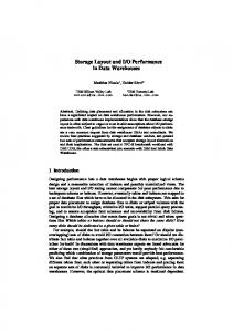
3 The Proposed Measures for Describing Data Characteristics The task of characterizing dataset for meta-learning is to capture the information about learning complexity on the given dataset. This information should enable the prediction of performance of learning algorithms. It should also be computable within a relative short time comparing to the whole learning process. In this section we introduce new measures to characterize the dataset by measuring a variety of properties of a decision tree induced from that dataset. The major idea here is to measure the model complexity by measuring the structure and size of decision tree, and use these measures to predict the complexity of other learning algorithms. We employed the standard decision tree learner, c5.0tree. There are several reasons for selecting decision trees. The major reason is that decision tree has been one of the most popularly used machine learning algorithms, and the induction of decision tree is deterministic, i.e. the same training set could produce the similar structure of decision tree. Definition. A standard tree induced with c5.0 (or possibly ID3 or c4.5) consists of a number of branches, one root, a number of nodes and a number of leaves. One branch is a chain of nodes from root to a leaf; and each node involves one attribute. The occurrence of an attribute in a tree provides the information about the importance of the associated attribute. The tree width is defined as the number of lengthways partitions divided by parallel nodes or leave from the leftmost to the rightmost nodes or leave. The tree level is defined as the breadth-wise partition of tree at each success branches, and the tree height is defined by the number of tree levels, as shown in Fig.1. The length of a branch is defined as the number of nodes in the branch minus one. level-1
F�
level-3 level-4
- root x2 c1
x1 c3
c1
TreeHigh
level-2
x1
- node - leaf x1,x2 - attributes c1,c2,c3 - classes
TreeWidth
Fig. 1. Structure of Decision Tree.
We propose, based on above notations, to describe decision tree in term of the following three aspects: a) outer-profile of tree; b) statistic for intra-structure: including tree levels and branches; c) statistic for tree elements: including nodes and attributes. To describe the outer-profile of the tree, the width of tree (treewidth) and the height of the tree (treeheight) are measured according to the number of nodes in each level and the number of levels, as illustrated in Fig.1. Also, the number of nodes (NoNode) and the number of leaves (NoLeave) are used to describe the overall property of a tree. In order to describe the intra-structure of the tree, the number of nodes at each level and the length of each branch are counted. Let us represent them with two vectors
Improved Dataset Characterisation for Meta-learning
145
denoted as NoinL=[v1,v2,…vl] and LofB=[L1,L2,….Lb] respectively, where vi is the number of nodes at the ith level, Lj is the length of jth branch, l and b is the number of levels (treeheight) and number of branches. Based on NoinL and LofB, the following four measures can be generated: The maximum and minimum number of nodes at one level:
maxLevel = max(v1,v 2 ,...v l ) minLevel = min(v1,v 2 ,...v l )
(1)
(As the minLevel is always equal to 1, it is not used.) The mean and standard deviation of the number of nodes on levels:
(∑ v ) l , l
meanLevel =
devLevel =
∑
l i =1
i =1 i
(2)
(vi − meanLevel ) 2 (l − 1)
The length of longest and shortest branches:
LongBranch = max(L1 , L2 ,...Lb )
(3)
ShortBranch = min(L1 , L2 ,...Lb ) The mean and standard deviation of the branch lengths:
(∑
b
meanBranch = devBranch =
∑
b j =1
j =1
)
Lj b ,
(4)
( L j − meanBranch) 2 (b − 1)
Besides the distribution of nodes, the frequency of attributes used in a tree provides useful information regarding the importance of each attribute. The times of each attribute is used in a tree represents by a vector NoAtt=[nAtt1, nAtt2, …. nAttm], where nAttk is the number of times the kth attribute is used and m is the total number of attributes in the tree. Again, the following measures are used: The maximum and minimum occurrence of attributes:
maxAtt = max(nAtt1,nAtt2 ,...nAttmm )
(5)
minAtt = min(nAtt1,nAtt2 ,...nAttmm ) Mean and standard deviation of the number of occurrences of attributes:
meanAtt =
devAtt =
∑
m
i =1
(∑
m
i =1
)
nAtt i m ,
(6)
(nAtti − meanAtt) 2 (m − 1)
As a result, a total of 15 meta-attributes (i.e., treewidth, treeheight, NoNode, NoLeave, maxLevel, meanLevel, devLevel, LongBranch, ShortBranch, meanBranch, devBranch, maxAtt, minAtt, meanAtt, devAtt) has been defined.
146
Y. Peng et al.
4 Experimental Evaluation In this section we experimentally evaluate the proposed data characteristics. In section 4.1 we describe our experimental set-up, in section 4.2 we compare our proposed meta-features with DCT and landmarking, and in section 4.3 we study the effect of meta-feature selection. 4.1 Experimental Set-up The meta-learning technique employed in this paper is an instance-based learning algorithm based ranking. Given a data mining problem (a dataset to analyze), the kNearest Neighbor (kNN) algorithm is used to select a subset with k dataset, whose characteristics are similar to the characteristics of the present dataset according to some distance function, from the benchmark datasets. Next, a ranking of their preference according to the the selected datasets is generated based on the adjusted ratio of ratios (ARR), a multicriteria evaluation measure that combines the accuracy and time. ARR has a parameter to enable the user to adjust the relative importance of accuracy and time according to his particular data mining objective. More details can be found in [26]. To evaluate a recommended ranking, we calculate its similarity to an ideal ranking obtained for the same dataset. The ideal ranking is obtained by estimating the performance of the candidate algorithms using 10-fold cross-validation. Similarity is measured using the Spearman’s rank correlation coefficient [29]. n n 6D2 2 2 2 (7) rs = 1− ,D = ∑i=1 Di = ∑i=1 (ri − ri ) 2 n(n − 1) where the
ri and r i are the predicted ranking and actual ranking for algorithm i re-
spectively. The bigger rs is, better of ranking result is, with rs = 1 if the ranking is same as the ideal ranking. In our experiments, a total of 10 learning algorithms, including c5.0tree, c5.0boost and c5.0rules [21], Linear Tree (ltree), linear discriminant (lindiscr), MLC++ Naive Bayes classifier (mlcnb) and Instance-based leaner (mlcib1) [11], Clementine Multilayer Perceptron (clemMLP), Clementine Radial Basis Function (clemRBFN) and rule learner (ripper), have been evaluated on 47 datasets, which are mainly from the UCI repository [4]. The error rate and time were estimated using 10-fold cross-validation. The leave-one-out method is used to evaluate the performance of ranking, i.e., the performance for ranking the 10 given learning algorithms for each dataset on the basis of the other 46 datasets. 4.2 Comparison with DCT and Landmarking The effect of new proposed meta-attributes (called DecT) has been evaluated on ranking of these 10 learning algorithms. In this section, we compare the ranking performance generated by DecT (15 meta-attributes) to that generated by DCT (25 meta-
Improved Dataset Characterisation for Meta-learning
147
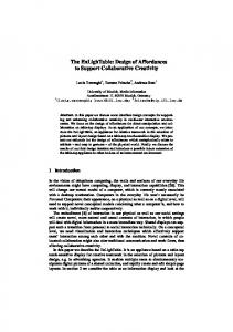
attributes) and Landmarking (5 meta-attributes). The used 25 DCT and 5 Landmarking meta-attributes are listed in the Appendix. The first experiment is performed to rank the given 10 learning algorithms on the 47 datasets, in which, the parameters k=10 (meaning the 10 most similar datasets are first selected from the 46 datasets in kNN algorithm), Kt=100 (meaning that we are willing to tread 1% in accuracy for a 100 times speed-up or slowdown [26]) is used. The ranking performance is measured with rs (Eq. (7)). The results of ranking performance of using DCT, landmarking and DecT are shown in Fig. 2. The overall average performance for DCT, Landmarking and DecT are 0.613875, 0.634945 and 0.676028 respectively, which demonstrates the improvement of DecT in ranking algorithms, comparing to DCT and Landmarking. � ��� ��� ��� ��� � ����
�
�
�
�� '&7
��
��
��
��
��
��
/DQGPDUNLQJ
��
��
'HF7
Fig. 2. Ranking performance for 47 datasets using DCT, landmarking and DecT.
In order to look in more detail at the improvement of DecT over DCT and Landmarking, we performed the experiment of ranking using different values of k and Kt. As stated in [26], the parameter Kt represents the relative importance of accuracy and execution time in selecting the learning algorithm (i.e., higher Kt means the accuracy is more important and time is less important in algorithm selection). Fig. 3 shows that for Kt={10,100,1000}, using DecT improves the performance comparing with the use of DCT and landmarking meta-attributes. ��� ��� ��� ��� ��� NW ��
NW ��� '&7
/DQGPDUNLQJ
NW ���� 'HF7
Fig. 3. The ranking performance for different values of Kt.
148
Y. Peng et al.
Fig. 4 shows the performance of ranking based on different zooming degree (different k), i.e., selecting different number of similar datasets, based on which the ranking is performed. From these results, we observe that 1) for all different values of k, DecT produces better ranking performance than DCT and landmarking; 2) best performance is obtained by selecting 10-25 datasets among 47 datasets. ���� ���� ���� ���� ���� N
�
N
�
N
�
N
�
N
�
'&7
N
��
N
��
N
��
N
/DQGPDUNLQJ
��
N
��
'HF7
Fig. 4. The ranking performance for different values of k.
4.3 Performing Meta-feature Selection The kNN-nearest neighbor (kNN) method, employed to select k datasets for ranking the performance of learning algorithms for the given dataset, is known to be sensitive to the irrelevant and redundant features. Using smaller number of features could help to improve the performances of kNN, as well as to reducing the time used in metalearning. In our experiments, we manually reduced the number of DCT meta-features from 25 to 15 and 8, and compare their results to those obtained based on the same number of DecT meta-features. The reduction for DCT meta-features is performed by removing the features thought to be redundant, and the features having a lot of nonappl (missing or error) values, and the reduction for DecT meta-features are performed by removing redundant features that are highly correlated. ���� ��� ���� ��� ���� ��� ���� ��� N
�
N
�
N
�
N
�
N
�
N
��
N
��
'&7��
'&7���
'HF7��
'HF7���
N
��
N
��
'&7���
Fig. 5. Results for reduced meta-features.
N
��
Improved Dataset Characterisation for Meta-learning
149
The ranking performances for these reduced meta-features are shown in Fig.5, in which DCT(8), DCT(15), DecT(8) represent the reduced 8, 15 DCT meta-features and 8 DecT meta-features, DCT(25) and DecT(15) represent the full DCT and DecT metafeatures respectively. From Fig.5, we can observe that feature selection did not significantly influence the performance of either DCT or DecT, and that the latter outperforms the former across the board.
5 Conclusions and Future Work Meta-learning strategy, under the framework of MetaL, aims at assisting the user in select appropriate learning algorithm for the particular data mining task. Describing the characteristics of dataset in order for estimating the performance of learning algorithm is the key to develop a successful meta-learning system. In this paper, we proposed new measures to characterise the dataset. The basic idea is to process the dataset using a standard tree induction algorithm, and then to capture the information regarding the dataset’s characteristics from the induced decision tree. The decision tree is generated using standard c5.tree algorithm. A total of 15 measures, which constitute the meta-attributes for meta-learning, have been proposed for describing different kind of properties of a decision tree. The proposed measures have been applied in ranking the learning algorithms based on accuracy and time. Extensive experimental results have illustrated the improvement of ranking performance by using the proposed 15 meta-attributes, compared to the 25 DCT and 5 Landmarking meta-features. In order to avoid the effect of redundant or irrelevant features on the performance of kNN learning, we also compared the performance of ranking based on the selected 15 DCT meta-features and DecT, and selected 8 DCT and DecT meta-features. The results suggest that feature selection does not significantly change performance of either DCT or DecT. In other experiments, we observed that the combination of DCT with DecT or Landmarking with DCT and DecT did not produce better performance than DecT. This is an issue that we are interested in further investigation. The major reason may come from the use of k-nearest neighbor learning in zooming based ranking strategy. One possibility is to test the performance of the combination of DCT, landmarking and DecT in other meta-learning strategies, such as best algorithm selection. Another interesting subject is to look at the change of shape and size of the decision tree along with the change of examples used in tree induction, as it will be useful if it is possible to capture the data characteristics based on sampled dataset. This is especially important for large datasets. Acknowledgements. this work is supported by the MetaL project (ESPRIT Reactive LTR 26.357).
150
Y. Peng et al.
References 1. 2.
3.
4. 5.
6. 7. 8.
9. 10.
11. 12.
13.
14. 15. 16. 17. 18.
C. E. Brodley. Recursive automatic bias selection for classifier construction. Machine Learning, 20:63-94, 1995. H. Bensusan, and C. Giraud-Carrier. Discovering Task Neighbourhoods through Landmark th Learning Performances. In Proceedings of the 4 European Conference on Principles of Data Mining and Knowledge Discovery. 325-330, 2000. H. Bensusan, C. Giraud-Carrier, and C. Kennedy. Higher-order Approach to Metalearning. The ECML’2000 workshop on Meta-Learning: Building Automatic Advice Strategies for Model Selection and Method Combination, 109-117, 2000. C. Blake, E. Keogh, C. Merz. www.ics.uci.edu/~mlearn/mlrepository.html. University of California, Irvine, Dept. of Information and Computer Sciences,1998. P. Brazdil, J. Gama, and R. Henery. Characterizing the Applicability of Classification Algorithms using Meta Level Learning. In Proceeedings of the European Conference on Machine Learning, ECML-94, 83-102, 1994. T. G. Dietterich. Approximate statistical tests for comparing supervised classification learning algorithms. Neural Computation, 10(7):1895-1924, 1998. E. Gordon, and M. desJardin. Evaluation and Selection of Biases. Machine Learning, 20(12):5-22, 1995. A. Kalousis, and M. Hilario. Model Selection via Meta-learning: a Comparative Study. In Proceedings of the 12th International IEEE Conference on Tools with AI, Vancouver. IEEE press. 2000. A. Kalousis, and M. Hilario. Feature Selection for Meta-Learning. In Proceedings of the 5th Pacific Asia Conference on Knowledge Discovery and Data Mining. 2001. C. Koepf, C. Taylor, and J. Keller. Meta-analysis: Data characterisation for classification and regression on a meta-level. In Antony Unwin, Adalbert Wilhelm, and Ulrike Hofmann, editors, Proceedings of the International Symposium on Data Mining and Statistics, Lyon, France, (2000). nd R. Kohavi. Scaling up the Accuracy of Naïve-bayes Classifier: a Decision Tree hybrid. 2 Int. Conf. on Knowledge Discovery and Data Mining, 202-207. (1996) M. Lagoudakis, and M. Littman. Algorithm selection using reinforcement learning. In Proceedings of the Seventeenth International Conference on Machine Learning (ICML2000), 511-518, Stanford, CA. (2000) C. Linder, and R. Studer. AST: Support for Algorithm Selection with a CBR Approach. th Proceedings of the 16 International Conference on Machine Learning, Workshop on Recent Advances in Meta-Learning and Future Work. 1999. D. Michie, D. Spiegelhalter, and C. Toylor. Machine Learning, Neural Network and Statistical Classification. Ellis Horwood Series in Artificial Intelligence. 1994. T. Mitchell. Machine Learning. MacGraw Hill. 1997. S. Salzberg. On Comparing Classifiers: Pitfalls to Avoid and a Recommended Approach. Data Mining and Knowledge Discovery, 1:3, 317-327, 1997. C. Schaffer. Selecting a Claassification Methods by Cross Validation, Machine Learning, 13, 135-143,1993. C. Schaffer. Cross-validation, stacking and bi-level stacking: Meta-methods for classification learning. In P. Cheeseman and R. W. Oldford, editors, Selecting Models from Data: Artificial Intelligence and Statistics IV, 51-59, 1994.
Improved Dataset Characterisation for Meta-learning
151
19. B. Pfahringer, H. Bensusan, and C. Giraud-Carrier. Tell me who can learn you and I can th tell you who you are: Landmarking various Learning Algorithms. Proceedings of the 17 Int. Conf. on Machine Learning. 743-750, 2000. 20. F. Provost, and B. Buchanan. Inductive policy: The pragmatics of bias selection. Machine Learning, 20:35-61, 1995. 21. J. R. Quinlan. C4.5: Programs for Machine Learning, Morgan Kaufman, 1993. 22. J. R. Quinlan. C5.0: An Informal Tutorial, RuleQuest, www.rulequest.com, 1998. 23. L. Rendell, R. Seshu, and D. Tcheng. Layered Concept Learning and Dynamically Varith able Bias Management. 10 Inter. Join Conference on AI. 308-314, 1987. th 24. C. Schaffer. A Conservation Law for Generalization Performance. Proceedings of the 11 International Conference on Machine Learning, 1994. 25. C. Soares. Ranking Classification Algorithms on Past Performance. Master’s Thesis, Faculty of Economics, University of Porto, 2000. 26. C. Soares. Zoomed Ranking: Selection of Classification Algorithms based on Relevant th Performance Information. Proceedings of the 4 European Conference on Principles of Data Mining and Knowledge Discovery, 126-135, 2000. 27. S. Y. Sohn. Meta Analysis of Classification Algorithms for Pattern Recognition. IEEE Trans. on Pattern Analysis and Machine Intelligence, 21, 1137-1144, 1999. 28. L. Todorvoski, and S. Dzeroski. Experiments in Meta-Level Learning with ILP. Proceedth ings of the 3 European Conference on Principles on Data Mining and Knowledge Discovery, 98-106, 1999. 29. A. Webster. Applied Statistics for Business and Economics, Richard D Irwin Inc, 779-784, 1992. 30. D. Wolpert. The lack of a Priori Distinctions between Learning Algorithms. Neural Computation, 8, 1341-1390, 1996. 31. D. Wolpert. The Existence of a Priori Distinctions between Learning Algorithms. Neural Computation, 8, 1391-1420, 1996. 32. H. Bensusan. God doesn’t always shave with Occam’s Razor - learning when and how to prune. In Proceedigs of the 10th European Conference on Machine Learning, 119--
124, Berlin, Germany, 1998.
Appendix DCT Meta-attributes: 1. Nr_attributes: Number of attributes. 2. Nr_sym_attributes: Number of symbolic attributes. 3. Nr_num_attributes: Number of numberical attributes. 4. Nr_examples: Number of records/examples. 5. Nr_classes: Number of classes. 6. Default_accuracy: The default accuracy. 7. MissingValues_Total: Total number of missing values. 8. Lines_with_MissingValues_Total: Number of examples having missing values. 9. MeanSkew: Mean skewness of the numerical attributes. 10. MeanKurtosis: Mean kurtosis of the numerical attributes.
152
Y. Peng et al.
11. NumAttrsWithOutliers: number of attributes for which the ratio between the alpha-trimmed standard-deviation and the standard-deviation is larger than 0.7 12. MStatistic: Boxian M-Statistic to test for equality of covariance matrices of the numerical attributes. 13. MStatDF: Degrees of freedom of the M-Statistic. 14. MStatChiSq: Value of the Chi-Squared distribution. 15. SDRatio: A transformation of the M-Statistic which assesses the information in the co-variance structure of the classes. 16. Fract: Relative proportion of the total discrimination power of the first discriminant function. 17. Cancor1: Canonical correlation of the best linear combination of attributes to distinguish between classes. 18. WilksLambda: Discrimination power between the classes. 19. BartlettStatistic: Bartlett’s V-Statistic to the significance of discriminant functions. 20. ClassEntropy: Entropy of classes. 21. EntropyAttributes: Entropy of symbolic attributes. 22. MutualInformation: Mutual information between symbolic attributes and classes. 23. JointEntropy: Average joint entropy of the symbolic attributes and the classes. 24. Equivalent_nr_of_attrs: ratio between class entropy and average mutual information, providing information about the number of necessary attributes for classification. 25. NoiseSignalRatio: Ratio between noise and signal, indicating the amount of irrelevant information for classification. Landmarking Meta-features: 1. Naive Bayes 2. Linear discriminant 3. Best node of decision tree 4. Worst node of decision tree 5. Average node of decision tree