Learning-Based Top-N Selection Query Evaluation over Relational Databases Liang Zhu*, Weiyi Meng** *
School of Mathematics and Computer Science, Hebei University, Baoding, Hebei 071002, China,
[email protected] ** Department of Computer Science, State University of New York at Binghamton, Binghamton, NY 13902, USA,
[email protected]
Abstract. A top-N selection query against a relation is to find the N tuples that satisfy the query condition the best but not necessarily completely. In this paper, we propose a new method for evaluating top-N selection queries against relational databases. This method employs a learning-based strategy. Initially, it finds and saves the optimal search spaces for a small number of random top-N queries. The learned knowledge is then used to evaluate new queries. Extensive experiments are carried out to measure the performance of this strategy and the results indicate that it is highly competitive with existing techniques for both low-dimensional and high-dimensional data. Furthermore, the knowledge base can be updated based on new user queries to reflect new query patterns so that frequently submitted queries can be processed most efficiently.
1 Introduction As pointed out in a number of recent papers [1, 4, 5, 6, 7, 9, 10, 15], it is of great importance to find the N tuples in a database table that best satisfy a given user query, for some integer N. This is especially true for searching commercial products on the Web. For example, for a Web site that sells used-cars, the problem becomes finding the N best matching cars based on a given car description. A top-N selection query against a relation/table is to find the N tuples that satisfy the query condition the best but not necessarily completely. A simple solution to this problem is to retrieve all tuples in the relation, compute their distances with the query condition using a distance function and output the N tuples that have the smallest distances. The main problem with this solution is its poor efficiency, especially when the number of tuples of the relation is large. Finding efficient strategies to evaluate top-N queries has been the primary focus of top-N query research. In this paper, we propose a new method for evaluating top-N selection queries against a relation. The main difference between this method and existing ones is that it employs a learning-based strategy. A knowledge base is built initially by finding the optimal (i.e., the smallest possible) search spaces for a small number of random top-N selection queries and by saving some related information for each optimal solution. *
This work is completed when the first author was a visitor at SUNY at Binghamton.
This knowledge base is then used to derive search spaces for new top-N selection queries. The initial knowledge base can be continuously updated while new top-N queries are evaluated. Clearly, if a query has been submitted before and its optimal solution is stored in the knowledge base, then this query can be most efficiently processed. As a result, this method is most favorable for repeating queries. It is known that database queries usually follow a Zipfian distribution [2]. Therefore, being able to support frequently submitted queries well is important for the overall performance of the database system. What is attractive about this method, however, is that even in the absence of repeating queries, our method compares favorably to the best existing methods with comparable storage size for storing information needed for top-N query evaluation. In addition, this method is not sensitive to the dimensionality of the data and it works well for both low-dimensional and high-dimensional data. The rest of the paper is organized as follows. In Section 2, we briefly review some related works and compare our method with the existing ones. In Section 3, we introduce some notations. In Section 4, we present our learning-based top-N query evaluation strategy. In Section 5, we present the experimental results. Finally in Section 6, we conclude the paper.
2. Related Work A large number of research works on the efficient evaluation of top-N selection queries (or N nearest-neighbors queries) are reported recently [1, 4, 5, 6, 7, 9, 10, 15]. Here we only review and compare with those that are most related to this paper. The authors of [10] use a probabilistic approach to query optimization for returning the top-N tuples for a given selection query. The ranking condition in [10] involves only a single attribute. In this paper, we deal with multi-attribute conditions. In [6], histogram-based approaches are used to map a top-N selection query into a traditional range selection query. In [1], the histogram-based strategies are extended to a new technique called Dynamic, expressed as dq(α) = dRq + α(dNRq - dRq). A significant weakness of histogram-based approaches is that their performance deteriorates quickly when the number of dimensions of the data exceeds 3 [1, 14]. Therefore, histogram-based approaches are suitable for only low-dimensional data in practice. In [7], a sampling-based method is proposed to translate a top-N query into an approximate range query. Unlike histogram-based approaches, this method is suitable for high-dimensional data and is easy to implement in practice. However, this method only provides an approximate answer to a given top-N query, i.e., it does not guarantee the retrieval of all of the top-N tuples. In addition, for large databases, this method may be inefficient. For example, for a relation with 1 million tuples and using a 5% sample set (as reported in [7]), 50,000 tuples need to be evaluated in order to find the approximate range query for a top-N query. Our learning-based method is fundamentally different from all existing techniques. It can learn from either randomly generated training queries or real user queries so it can adapt to changes of query patterns. Furthermore, it delivers good performance for both low-dimensional and high-dimensional data.
3 Problem Definition Let ℜ
n
be a metric space with distance (or, metric) function d(.,.), where ℜ is the n
real line. Suppose that R ⊆ ℜ is a relation (or dataset) with M tuples and n attributes (A1, …, An). A tuple t ∈ R is denoted by t = (t1, …, tn). Consider a point (query) Q = n
(q1,…, qn)∈ ℜ . A top-N selection query, or top-N query for short, is to find a sorted set of N tuples in R that are closest to Q according to the given distance function. The results of a top-N query are called top-N tuples. Suppose Q = (q1,…, qn) is a top-N query and r > 0 is a real number. We use S(Q, r) to denote the n-square ∏ n [ q i − r , q i + r ] centered at Q with side length 2r. Our i =1
goal is to find a search distance r as small as possible such that S(Q, r) contains the top-N tuples of Q according to the given distance function. We use S(Q, r, N) to denote this smallest possible n-square and the corresponding r is called the optimal search distance for the top-N query Q. Some example distance functions are [1, 7, 15]: Summation distance (i.e., L 1 -norm or Manhattan distance): d 1 (x, y) =
∑
n i =1
| xi − yi | .
Euclidean distance (i.e., L 2 -norm distance): d 2 (x, y) =
∑
n i =1
( xi − yi ) 2 .
Maximum distance (i.e., L ∞ -norm distance): d ∞ (x, y) = max {| x i − y i |} . 1≤ i ≤ n
Frequently, it is not suitable to apply a distance function to the values of different attributes directly due to the unit/scaling difference of the values in different attributes. For example, when buying a used car, a 100-dollar difference in price is probably more significant than a 100-mile difference in mileage. This can be resolved by multiplying appropriate importance/scaling factors to the raw distances based on the values of different attributes [9, 15]. Without loss of generality, in this paper, we assume that all attributes are of the same importance for ranking tuples so that the distance functions can be applied directly.
4 Learning-based Top-N Query Evaluation In this section, we introduce our learning-based method for top-N query evaluation. First, keep track of frequently submitted queries and save the evaluation strategies for these queries in a knowledge base. Next, for each newly submitted query, if its evaluation strategy has been saved or it is similar to some queries whose evaluation strategies have been saved, then derive an evaluation strategy for the new query from the saved relevant strategy/strategies. In this paper, we study issues related to this method. 4.1 Query Information to Save Initially, the knowledge base is empty. When a new query arrives at the system, an existing method such as the one proposed in [1] or in [7] is employed to evaluate the query. Let Q = (q1, …, qn) be the query and ti = (ti1, …, tin), 1 ≤ i ≤ N, be the top-N tu-
ples, respectively, then the search distance of the smallest n-square is r = max {d ∞ (Q, t i )} = max {max {| q j − t ij |}} . When the smallest n-square is ob1≤ i≤ N
1≤ i ≤ N
1≤ j ≤ n
tained, several pieces of information are collected and saved. For a top-N query Q, let r be the search distance of S(Q, r, N) – the smallest n-square that contains the top-N tuples of Q, f denote the frequency of S(Q, r, N), i.e., the number of tuples in S(Q, r, N) (obviously N ≤ f ), c denote the number of times that Q has been submitted, and d denote the most recent time when Q was submitted. The information that we will keep for each saved query Q is represented as ζ(Q) = (Q, N, r, f, c, d) and it is called the profile of the query. After the system has been used for sometime, a number of query profiles are created and saved in the knowledge base. Let P = {ζ 1 , ζ 2 , …, ζ m } denote the set of all query profiles, i.e., the knowledge base, maintained by the system. Queries in P will be called profile queries. Generally, profiles should be kept only for queries that are frequently submitted recently as reflected by the values of c and d in each profile. In our implementation, the initial knowledge base is not built based on real user queries. Instead, it is based on randomly selected queries from a possible query space (see Section 5 for more details). 4.2 New Query Evaluation When a newly submitted top-N query Q is received by the system, we need to find an appropriate search distance r for it. In a system that does not store query profiles, this query will be processed just like any new query and the methods discussed in [1, 7] may be used to find r. When query profiles are stored, it becomes possible to obtain the r for some new user queries from these profiles. 4.2.1 Determining the search distance r The details of obtaining the search distance r for a new query are described below.
Figure 1. Q = Q′.
Figure 2. Q ∈ S(Q′, r′, N’ ). Figure 3. Q ∉ S(Q′, r′, N’ )
First we identify Q′ = ( q 1′ , q ′2 ,..., q ′n ) from P that is the closest to Q under the distance function d(.,.). The following cases exist. 1. d(Q, Q′ ) = 0, i.e., Q′ = Q . In this case, find all profiles in P whose query point is Q′, but have different result size N, say, N1< N2 < …< Nk. An example of a 2dimension case is depicted in Figure 1, where squares of solid-lines represent the search spaces of profile queries (i.e., those in P) and the square of dotted-lines represents the search space of the new query Q. We now consider three subcases.
a. There is N′ ∈ {N1, N2, …, Nk} such that N = N′. That is, there is a top-N query in P that is identical to the new query in both the query point and result size. In this case, let r := r′, where r′ is from the profile ζ′ = (Q′, N′, r′, f′, c′, d′ ). b. There is no N′ ∈ {N1, N2, …, Nk} such that N = N′ but there is N′ ∈ {N1, N2, …, Nk} such that N′ > N and it is the closest to N among N1, N2, …, Nk (Figure 1). In this case, let r := r′ to guarantee the retrieval of all the top-N tuples for Q. c. Nk < N. In this case, we assume that the search space for Q has the same local distribution density as that for Q′. Based on this assumption, we have N/(2r)n = Nk/(2rk)n. As a result, we let r := ( n N N k )rk. If not enough top-N tuples are retrieved, a larger r will be used (see Section 4.2.2). 2. d(Q, Q′ ) ≠ 0, i.e., Q′ ≠ Q. We consider two subcases. a. Q is in the search space S(Q′, r′, N′ ) of Q′ . Find out all query points in P whose search spaces contain Q. Let these query points be (Q1, …, Qk) (see Figure 2). To estimate the search distance r for Q, we first use a weighted average of the local distribution densities of the search spaces for Q1, …, Qk to estimate the local density of search space for Q. The weight wi for the search space corresponding to Qi is computed based on its size and the distance between Qi and Q. Weight wi is an increasing function of the size of the search space and a decreasing function of the distance. In this paper, wi is computed by the following formula: wi = v(S(Qi, ri, Ni)) * 1/(d(Q, Qi))α where α is a parameter and α = 3n/4 is a good value based on our experiments. Let ρi = fi /(2 ri)n be the local density of the search space for Qi. Then the local density of the search space for Q is estimated by: k
k
ρ = (∑ i =1 wi ρ i ) / (∑ i =1 wi). Based on the above ρ, we estimate the search distance r to be ( n 2 N / ρ )/2. Note that to increase the possibility that all of the top-N tuples for Q are retrieved, we replaced N by 2N in the estimation for r (i.e., aim to retrieve 2N tuples). b. Q is not in the search space S(Q′, r′, N′ ) of Q′ (see Figure 3). Let h := d(Q, Q′ ) be the distance between Q and Q′. Construct an n-square S(Q, h) and let (Q1, …, Qk) be all the query points in P whose search spaces intersect with S(Q, h). Obviously, k ≥ 1 as Q′ is in this query set. Now the same technique used above in step 2.a is used to estimate the search distance r for Q. The search distance r obtained above (2.a and 2.b) may sometimes be either too small or too large. To remedy this, the following adjustments to r are implemented. The following two cases are considered. (1) N = N′ . (i) If r < r′ or r < d(Q, Q′ ), then r may be too small. We use the following formula to adjust r: r =max(r_Median, r_Mean, r)/2 + (r′ +d(Q, Q′ ))/2 where r_Median = ( n 2 N / N median ) rmedian , rmedian is the search distance of the search space whose density is the median among all search spaces in P, and N median is the N value of the corresponding profile; r_Mean =
(
n
2 N / ρ mean )/2 and ρ mean is the average of all the densities of the search
spaces in P. (ii) If r > r′ + d(Q, Q′ ), then r is too large as r = r′ + d ∞ (Q, Q′ ) can already guarantee the retrieval of all the top-N tuples of Q. In this case, we simply lower r to r′ + d(Q, Q′ ). (2) N ≠N′ . This is handled in a similar manner as in case (1) except that a constant factor λ = n N / N ′ is utilized to take into consideration the difference between N and N′. (i) If r < λ r′ or r < d(Q, Q′ ), then r := max(r_Median, r_Mean, r)/2 + (λr′ + d(Q, Q′ ))/2. (ii) If r > λ r′ + d(Q, Q’ ), then r := λ r′ + d(Q, Q′ ). 4.2.2 Query Mapping Strategies For a given top-N query Q = (q1,…, qn), to retrieve all tuples in S(Q, r), one strategy is to map each top-N query to a simple selection range query of the following format [1]: SELECT * FROM R WHERE (q1 – r ≤ A1 ≤ q1 + r) AND … AND (qn – r ≤ An ≤ qn + r) If the query returns ≥ N results, sort them in non-descending distance values and output the top N tuples. A potential problem that needs to be handled is that the estimated search distance r is not large enough. In this case, the value of r needs to be increased to guarantee that there are at least N tuples in S(Q, r). One solution to this problem is provided below. Choose N query points in P, which are closest to the top-N query Q, and sort them in ascending order of their distances with Q with respect to the used distance function d(.,.). Let the order be Q1, …, QN and their corresponding profiles be ζ 1 , ζ 2 , …, ζ N . There exists a number h, 1 < h ≤ N, such that N1 + … + Nh ≥ N. During the computation of the sum, if S(Qi, ri, Ni) ∩ S(Qj, rj, Nj) ≠ φ , then Ni + Nj in the above sum was replaced by max{Ni, Nj} to ensure that the search spaces of the first h queries in (Q1, …, QN) contain at least N unique tuples. Let r := max {d(Q, Qi) 1≤i≤ h
+ ri}.Thus, by using this r as the search distance for Q to generate the restart query, the restart query will guarantee the retrieval of all the top-N tuples for Q. If there is a histogram over the relation R, by using dNRq in [1], the search distance r for the restart query can be obtained as follows. If the sum of all N’s in P is less than N, then set r to be dNRq. Otherwise, find the number h as mentioned above and let r := min{ max {d(Q, Qi) + ri}, dNRq}. 1≤i≤ h
5
Experimental Results
5.1 Data Sets and Preparations All of our experiments are carried out using Microsoft's SQL Server 7.0 on a PC. To facilitate comparison, the same datasets and parameters used in [1] and [7] are used in
this paper. These datasets include data of both low dimensionality (2, 3, and 4 dimensions) and high dimensionality (25, 50, and 104 dimensions). For low-dimensional datasets, both synthetic and real datasets used in [1] are used. The real datasets include Census2D and Census3D (both with 210,138 tuples), and Cover4D (581,010 tuples). The synthetic datasets are Gauss3D (500,000 tuples) and Array3D (507,701 tuples). In the names of all datasets, suffix KD indicates that the dataset has K dimensions. For high-dimensional datasets, real datasets derived from LSI are used in our experiments. They have 20,000 tuples and the same 25, 50 and 104 attributes as used in [7] are used to create datasets of 25, 50 and 104 dimensions, respectively. Each experiment uses 100 test queries (called a workload). The workloads follow two distinct query distributions, which are considered representatives of user behaviors [1]: Biased: Each query is a random existing point in the dataset used. Uniform: The queries are random points uniformly distributed in the dataset used. The uniform workloads are only used for low-dimensional datasets to compare the results with those of [1]. For convenience, we report results based on a default setting. This default setting uses a 100-query Biased workload, N = 100 (i.e., retrieve top 100 tuples for each query) and max is the distance function. When a different setting is used, it will be explicitly mentioned. The most basic way of processing a top-N query is the sequential scan method [4, 5]. In this paper, we compare the following four top-N query evaluation techniques: Optimum technique [1]. As a baseline, we consider the ideal technique that uses the smallest search space containing the actual top-N tuples for a given query. The smallest search space is obtained using the sequential scan technique in advance. Histogram-based techniques [1]. We only cite the results produced by the dynamic (Dyn) mapping strategy described in [1] for comparison purpose. Dyn is the best among all histogram-based techniques studied in [1]. Sampling-based technique [7]. In this paper, we only cite the experimental results produced by the parametic (Para) strategy described in [7]. The Para strategy is the best of all sampling-based strategies discussed in [7]. Learning-based (LB) technique. This is our method described in Sections 4. For a given dataset D, the knowledge-base (or profile set) P is constructed as follows. First, a set of random tuples from D is selected. The size of the random tuple set is decided such that the size of P does not exceed the size of the histogram or the size of the sampling set when the corresponding method is being compared. For each query point chosen for P, the sequential scan technique is used to obtain its profile during the knowledge-base construction phase. For easy comparison, we use the following performance metrics used in [1] in this paper. Percentage of restarts: This is the percentage of the queries in the workload for which the associated selection range query failed to retrieve the N best tuples, hence leading to the need of a restart query. When presenting experimental results, Method(x%) is used to indicate that when evaluation strategy Method is used, the percentage of restart queries is x%. For example, LB(3%) means that there are 3% restart queries when the learning-based method is used. Percentage of tuples retrieved: This is the average percentage of tuples retrieved from the respective datasets for all queries in the workload. When at least N tuples are retrieved, lower percentage of tuples retrieved is an indication of better efficiency. We
report SOQ (Successful Original Query) percentages and IOQ (Insufficient Original Query) percentages. The former is the percentage of the tuples retrieved by the initial selection range query and the latter is the percentage of the tuples retrieved by a restart query when the initial query failed to retrieve enough tuples. 5.2 Performance Comparison 5.2.1 Comparison with Dyn The experimental results that compared Dyn and Para were reported for lowdimensional datasets and for both Biased and Uniform workloads in [1] and the differences between the two methods are very small. Therefore, it is sufficient to compare LB with one of these two methods for low-dimensional datasets.
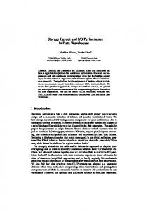
(a) Biased Workloads
(b) Uniform Workloads
Figure 4. Comparison of LB and Dyn
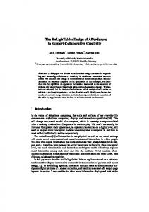
(a) Eucl-distance, 25, 50, 104 dimensions
(b) Lsi50D, Sum, Eucl and Max
Figure 5. Comparison of LB and Para
Figure 4 compares the performance of LB and that of Dyn for different datasets and for both Biased and Uniform workloads. From Figure 4(a), it can be seen that when Biased workloads are used, for datasets Gauss3D and Census3D, LB outperforms Dyn significantly; for Array3D, Census2D and Cover4D, LB and Dyn have similar performance. For Uniform workloads (Figure 4(b)), LB is significantly better than Dyn for 4 datasets and is slightly better for 1 dataset. However, LB has much higher restart percentages for Gauss3D and Cover4D (95% and 31%, respectively).
5.2.2 Comparison with Para for High-Dimensional Datasets Note that the Para method does not aim to guarantee the retrieval of all top-N tuples. In [7], results for top-20 (i.e., N=20) queries when retrieving 90% (denoted Para/90) and 95% (denoted Para/95) were reported. In contrast, LB guarantees the retrieval of all top-N tuples for each query. Figure 5 compares the performances of LB and Para for top-20 queries [7]. When Euclidean distance function is used, LB slightly underperforms Para/95 for 25- and 50-dimensional data but significantly outperforms Para/95 for 104-dimensional data. Figure 5(b) shows the results using different distance functions for 50-dimensional data. For the most expensive sum function, LB is significantly better than Para/95; for Euclidean distance function, Para/95 is slightly better than LB, and for the max function, Para/95 is significantly better than LB. 5.3 Additional Experimental Results for LB We carried out a number of additional experiments to gain more insights regarding the behavior of the LB method. In this section, we report the results of these experiments. Effect of Different Result Size N. Based on dataset Census2D, we construct 4 different knowledge bases using top-50, top-100, top-250 and top-1000 queries, respectively. For each knowledge base, the number of queries used is the same (1,459 queries). These knowledge bases are then used to evaluate a test workload of 100 top-100 queries. Our results indicate that using the knowledge bases of top-50 and top-100 queries yields almost the same performance. The best and the worst performances are obtained when the knowledge base of top-250 queries and that of top-1000 queries are used, respectively. Effect of Different Values of N. In the second set of experiments, we use some top-100 queries to build a knowledge base for each of the 5 low-dimensional datasets. 178, 218 and 250 queries are used to build the knowledge base for 2-, 3- and 4dimensional datasets, respectively. Each knowledge base is then used to evaluate a workload of top-50, top-100, top-250 and top-1000 queries. Overall, the results are quite good except when top-1000 queries are evaluated. But even for top-1000 queries, on the average, no more than 2% of the tuples are retrieved in the worst-case scenario. For this experiment, our results indicate that the LB method performs overall much better than the Dyn method. For example, in only two cases, more than 1% of the tuples are retrieved by LB, but in Figure 22(b) in [1], there are 10 cases where more than 1% of the tuples are retrieved. Effect of Different Distance Functions. The effectiveness of the LB method may change depending on the distance function used. Our experimental results using various low-dimensional datasets indicate that the LB method produces similar performance for the three widely used distance functions (i.e., max, Euclidean and sum). By comparing our results with Figure 21(b) in [1], we find that the LB method significantly outperforms the Dyn method for datasets Gauss3D, Census3D and Cover4D; for the other two datasets, namely Array3D and Census2D, the two methods have similar performance.
6 Conclusions In this paper, we proposed a learning-based strategy to translate top-N selection queries into traditional selection queries. This technique is robust in several important aspects. First, it can cope with a variety of distance functions. Second, it does not suffer the much feared “dimensionality curse” as it remains effective for high-dimensional data. Third, it can automatically adapt to user query patterns so that frequently submitted queries can be processed most efficiently. We carried out extensive experiments using a variety of datasets of different dimensions (from 2 to 104). These results demonstrated that the learning-based method compares favorably with the current best processing techniques for top-N selection queries. Acknowledgments: The authors would like to express their gratitude to Nicolas Bruno [1] and Chung-Min Chen [7] for providing us some of the test datasets used in this paper and for providing us some experimental results of their approaches that made it possible for us to compare with their results directly in this paper.
References 1. N. Bruno, S. Chaudhuri, and L. Gravano. Top-k Selection Queries over Relational Databases: Mapping Strategies and Performance Evaluation, ACM Transactions on Database Systems, 27 (2), 2002, 153–187. 2. N. Bruno, S. Chaudhuri and L. Gravano. STHoles: A Multidimensional Workload-Aware Histogram. ACM SIGMOD Conference, 2001. 3. N. Bruno, L. Gravano, and A.Marian. Evaluating Top-k Queries over Web-Accessible Databases. 18th IEEE International Conference on Data Engineering, 2002. 4. M. Carey, and D. Kossmann. On saying “Enough Already!” in SQL. ACM SIGMOD Conference, 1997. 5. M. Carey, and D. Kossmann. Reducing the braking distance of an SQL query engine. International Conference on Very Large Data Bases. 1998. 6. S. Chaudhuri, and L. Gravano. Evaluating top-k selection queries. International Conference on Very Large Data Bases, 1999. 7. C. Chen, and Y. Ling, A sampling-based estimator for top-k selection query. 18th International Conference on Data Engineering, 2002. 8. C. Chen and N. Roussopoulos. Adaptive selectivity estimation using query feedback. ACM SIGMOD Conference, 1994, 161–172. 9. Y. Chen, and W. Meng. Top-N Query: Query Language, Distance Function and Processing Strategies. International Conference on Web-Age Information Management, 2003. 10. D. Donjerkovic, and R. Ramakrishnan. Probabilistic optimization of top N queries. International Conference on Very Large Data Bases, 1999. 11. R. Fagin. Combining fuzzy information from multiple systems. ACM Symposium on Principles of Database Systems, 1996, 216-226. 12. R. Fagin. Fuzzy queries in multimedia database systems. ACM Symposium on Principles of Database Systems, 1998. 13. R. Fagin, A. Lotem, and M. Naor. Optimal aggregation algorithms for middleware. ACM Symposium on Principles of Database Systems, 2001. 14. J. Lee, D. Kim, and C. Chung. Multi-dimensional Selectivity Estimation Using Compressed Histogram Information. ACM SIGMOD Conference, 1999, 205-214. 15. C. Yu, G. Philip, and W. Meng. Distributed Top-N Query Processing with Possibly Uncooperative Local Systems. VLDB, Berlin, Germany, September 2003, 117-128.