an R package and a C/C++ library with a MATLAB front-end that permit parallelized, fast and ... libstable: α-Stable Distributions in R, C/C++, MATLAB one hand, to the ... interface and statistical tools of MATLAB and R environments. The rest of ...
JSS
Journal of Statistical Software June 2017, Volume 78, Issue 1.
doi: 10.18637/jss.v078.i01
libstable: Fast, Parallel, and High-Precision Computation of α-Stable Distributions in R, C/C++, and MATLAB Javier Royuela-del-Val
Federico Simmross-Wattenberg
University of Valladolid
Universidad de Valladolid
Carlos Alberola-López Universidad de Valladolid
Abstract α-stable distributions are a family of well-known probability distributions. However, the lack of closed analytical expressions hinders their application. Currently, several tools have been developed to numerically evaluate their density and distribution functions or to estimate their parameters, but available solutions either do not reach sufficient precision on their evaluations or are excessively slow for practical purposes. Moreover, they do not take full advantage of the parallel processing capabilities of current multi-core machines. Other solutions work only on a subset of the α-stable parameter space. In this paper we present an R package and a C/C++ library with a MATLAB front-end that permit parallelized, fast and high precision evaluation of density, distribution and quantile functions, as well as random variable generation and parameter estimation of α-stable distributions in their whole parameter space. The described library can be easily integrated into third party developments.
Keywords: α-stable distributions, numerical calculation, parallel processing.
1. Introduction α-stable distributions are a family of probability distributions that permit adjustable levels of heavy tails and skewness and include distributions such as Gaussian, Cauchy and Lévy as particular cases. They were first introduced by Lévy (1925) and have since been applied in many research fields. The increasing interest in α-stable distributions is due, on the
2
libstable: α-Stable Distributions in R, C/C++, MATLAB
one hand, to the empirical evidence that they properly describe the behavior of real data exhibiting impulsiveness or strong asymmetries; on the other hand, the generalized central limit theorem (Samorodnitsky and Taqqu 1994) states that the normalized sum of independent and identically distributed random variables with finite or infinite variance converges, if so, to an α-stable distribution. This result provides theoretical support when the data under study can be interpreted as the superposition of many independent sources. This way, Mandelbrot and Wallis (1968) model precipitation data as α-stable measurements, Fama (1965) and Borak, Misiorek, and Weron (2011) use them to predict stock prices and asset returns, Simmross-Wattenberg, Asensio-Pérez, de-la Higuera, Martín-Fernández, Dimitriadis, and Alberola-López (2011) and Willinger, Taqqu, Sherman, and Wilson (1997) show that the marginal distribution of aggregated network traffic may be accurately modeled by stable laws; in addition, Vegas-Sánchez-Ferrero, Simmross-Wattenberg, Martín-Fernández, Palencia, and Alberola-López (2012) use them to characterize speckle noise in medical ultrasonic data, Salas-Gonzalez, Górriz, Ramírez, Schloegl, Lang, and Ortiz (2013) model white and gray matter of the brain in magnetic resonance imaging as α-stable random variables and Gonchar, Chechkin, Sorokovo˘ı, Chechkin, Grigor’eva, and Volkov (2003) characterize ion current fluctuations in plasma physics as being α-stable. All these phenomena share the common property of being markedly impulsive in nature and, in many cases, strongly asymmetrical, so α-stable distributions emerge as natural candidates to work with. However, α-stable distributions are not limited to modeling natural phenomena. Li, Samorodnitsk, and Hopcroft (2013) describe how to use them to compute distance (or similarity) in high-dimensional data and Li, Zhang, and Zhang (2014) use them to recover sparse signals under compressed sensing theory. Both of these proposals, in turn, have many applications on their own and the list is far from complete. The major drawback for the application of α-stable models is the lack of closed analytical expressions for their probability density function (PDF) or cumulative distribution function (CDF) except in particular cases, which makes the application of numerical methods a must. Besides, the non-existence of moments of order two or higher (except in the Gaussian case) increases the difficulty in estimating their parameters to fit real data. Several authors have addressed both the numerical evaluation of the PDF or CDF of α-stable distributions (Nolan 1997; Mittnik, Doganoglu, and Chenyao 1999a; Belov 2005; Menn and Rachev 2006; Górska and Penson 2011) and the estimation of their parameters (Fama and Roll 1971; Koutrouvelis 1981; McCulloch 1986; Mittnik, Rachev, Doganoglu, and Chenyao 1999b; Nolan 2001; Fan 2006; Salas-Gonzalez, Kuruoglu, and Ruiz 2009) and have proposed different methods and algorithms for these purposes (details are discussed in Section 2). Some authors also provide implementations of their own or relying on others’ methods, offering software solutions or packages in various common computer languages. However, some of these solutions are not fully operational in their public domain versions and do not take advantage of multi-core processors (Nolan 2006), have limited accuracy (Belov 2005; Menn and Rachev 2006) or take a computation time that makes results unaffordable for several practical applications (Veillete 2010; Liang and Chen 2013). In this paper we present an R (R Core Team 2017) package and a C/C++ library with a MATLAB front-end (The MathWorks Inc. 2013) that permit parallelized, fast and high precision evaluation of density and distribution functions, random variable generation and parameter estimation in α-stable distributions. The library can be easily integrated in third party developments to be used by practitioners. Its utilization in MATLAB and R is straightforward
3
Journal of Statistical Software
and takes advantage of both the high efficiency of the compiled C/C++ code and the familiar interface and statistical tools of MATLAB and R environments. The rest of the paper is organized as follows. In Section 2, currently proposed algorithms and methods to numerically evaluate the density and distribution functions of α-stable distributions are described, as well as reported methods to estimate their parameters. In Section 3, the developed library and its functionality are presented. The results obtained with the library are discussed in Section 4. In Section 5, the usage of the proposed library is described. Finally, Section 6 describes main conclusions and further work possibilities derived from this work.
2. Numerical methods in α-stable distributions α-stable distributions are typically described by their characteristic function (CF) due to the fact that no closed expressions exist for the general case. Let Φ(t) = exp[Ψ(t)] denote this function with (Samorodnitsky and Taqqu 1994): � � � −|σt|α 1 − iβ tan πα sign(t) + iµt, α 6= 1, 2 Ψ(t)= � � −|σt| 1 + iβ π2 sign(t) ln (|t|) + iµt, α = 1, (
where sign(t)
(1)
1, t > 0, 0, t = 0, −1, t < 0.
=
The four parameters above are (1) the stability index α ∈ (0, 2], (2) the skewness parameter β ∈ [−1, 1], (3) the scale parameter σ > 0 and (4) the location parameter µ ∈ R. An α-stable distribution is referred to as standard if σ =√1 and µ = 0. When α = 2 the distribution becomes normal with standard deviation σ/ 2 and mean µ (β becomes irrelevant). The Cauchy distribution results from setting α = 1 and β = 0 with scale parameter σ and location parameter µ, and the Lévy distribution when α = 0.5 and β = 1. These are the only cases for which the PDF can be expressed analytically. Otherwise, the PDF has to be calculated numerically. The next subsections discuss different methods proposed in the literature to obtain the PDF and CDF, to estimate the parameters of α-stable distributions and to generate samples of an α-stable random variable.
2.1. Numerical computation of α-stable distributions The PDF and CF of any probability function are related via the Fourier inversion formula given by 1 f (x) = 2π
Z
+∞ −itx
φ(t)e −∞
1 dt = 2π
Z
+∞
eψ(t)−itx dt.
(2)
−∞
When substituting Equation 1 in Equation 2 the resulting integral cannot be, as a rule, solved analytically; therefore it must be evaluated by numerical methods. To this end, the wellknown fast Fourier transform (FFT) provides an algorithm to efficiently evaluate the previous integral. Mittnik et al. (1999a) apply the FFT directly to calculate the PDF. However, this approach suffers from several important drawbacks. First, the algorithm provides the value
4
libstable: α-Stable Distributions in R, C/C++, MATLAB
of the integral on a set of evenly spaced points of evaluation. This is not valid for some applications, where the PDF or CDF must be evaluated at some specific set of points. A posterior step of interpolation is then required, which introduces additional computational costs and reduces precision. Second, the method is only suitable for α close to 2, for which the tails of the distribution decay more quickly. When α is small, the tails decay very slowly and the aliasing effect becomes more noticeable, thus reducing the achievable precision. Experimentally, the committed absolute error is in the order of 10−5 , but relative error goes as high as 10−2 . Menn and Rachev (2006) propose a method based on a refinement of the FFT to increase precision in the central part of the PDF. The tails of the distribution are calculated via the Bergström asymptotic series expansion (Zolotarev 1986), which provides an alternative expression as an infinite sum of decaying terms. This way they achieve relative precision of about 10−4 , but this precision heavily depends on the values of α and β and the method is only applicable when α > 1. Górska and Penson (2011) follow a different approach and obtain explicit expressions for the PDF and CDF as series of generalized hypergeometric functions. However, the expressions involved in the calculation are expensive to evaluate and the results are only valid for some rational values of the parameters α and β, so they are not valid for the whole parameters space. When compared with the FFT, direct integration of the expression in Equation 2 by numerical quadrature initially implies a higher computational cost, but evaluation can be performed at any desired set of points without the need of additional interpolation steps and there is no restriction on the values of the distribution parameters. This method has been implemented by Nolan (1999)1 . However when α is small the integrand oscillates very quickly and its amplitude decays slowly along the infinite integration interval, which limits the achievable precision even when many evaluations of the integrand are used. According to the author, the method results are valid only for α > 0.75 and it achieves a precision in the order of 10−6 . Similar results have been obtained later by Belov (2005), where the infinite integrand interval is divided in two (one bounded and the other infinite) and two quadrature formulae are applied. In order to overcome the previous difficulties, Nolan (1997) obtains a new set of equations from the original ones by means of an analytic extension of the integrand to the complex plane. This way, a continuous, bounded, non-oscillating integrand is obtained. Moreover, the integration interval becomes finite. The expressions obtained allow the author to achieve, by numerical quadrature, a relative accuracy in the order of 10−14 in most of the parameter space. For numerical convenience, a slightly different parameterization of the distribution is employed, based on Zolotarev (1986) M parameterization. The modification introduced consists in a shift of the distribution along the abscissae axis in order to avoid the discontinuity of the distribution at α = 1. In this paper, we denote the change in parameterization by the subindex 0 and the resulting CF is given by Φ0 (t) = exp[Ψ0 (t)], where (
Ψ0 =
1−α−1 +iµ t, α 6= 1, −|σt|αh 1+iβtan πα 0 2 sign(t) |σt| i 2 −|σt| 1+iβ π sign(t) ln (|σt|) +iµ0 t, α = 1.
�
�
��
(3)
The parameters α, β and σ keep their previous meaning while the original and modified 1 Although finally published in 1999, this article is already cited in Nolan (1997) as a “to appear in” reference, so the described software therein is earlier than 1997.
5
Journal of Statistical Software location parameters µ and µ0 are related according to (
µ=
µ0 − β tan απ 2 σ, α 6= 1, 2 µ0 − β π σ ln(σ), α = 1. �
(4)
With this modification, the resulting distribution is continuous in its four parameters, which is convenient when estimating the parameters of the distribution or approximating its PDF or CDF.
2.2. Parameter estimation of α-stable distributions As previously explained, the lack of closed expressions for the PDF or CDF of α-stable distributions implies a major drawback when estimating their parameters. Therefore, the techniques employed for the estimation usually rely on numerical evaluations of these functions or, alternatively, are based on other properties of the distributions. Several methods can be found in the related literature. Hill (1975) proposes the estimation of the α parameter by linear regression on the right tail of the empirical distribution. However, in many practical cases the method is not applicable because of the high number of samples needed to detect the tail behavior. McCulloch (1986) proposes an algorithm to estimate the four parameters of the α-stable distribution simultaneously from sample quantiles and tabulated values. The resulting estimator has a very low computational cost but a low accuracy as well. However, it can be conveniently used to provide initial estimates for other methods. Koutrouvelis (1981) departs from the empirical CF to obtain, by means of recursive linear regressions on its log-log plot, estimators for α and σ in a first step and for β and µ in a second one. The method implies a higher computational cost than the quantile method, but yields more accurate results. Maximum likelihood (ML) estimation is considered the most accurate estimator available for α-stable distributions (Borak et al. 2011). However, numerical methods to both approximate the PDF and to maximize the likelihood of the sample must be used, which implies a very high computational cost due to the numerous PDF evaluations required to maximize the likelihood in the four-dimensional parameter space. However, increasing computer capabilities and the use of precalculated values of the PDF make the use of this method possible in certain applications (Nolan 2001).
2.3. Generation of α-stable random variables Given the lack of closed expressions for the CDF or its inverse (the quantile function, CDF−1 ), the simulation of α-stable distributed random variables cannot be achieved easily from a uniform random variable. Chambers, Mallows, and Stuck (1976) provided a direct method to generate an α-stable random variable by means of the transformation of an exponential and a uniform random variable. The method proposed lacked a theoretical demonstration until Weron (1996) gave an explicit proof and slightly modified the original expressions. The resulting method is regarded as the fastest and the most accurate available (Weron 2004). Based on the methods described so far, several software tools are currently available. The program STABLE (Nolan 2006) employs Nolan’s expressions (Nolan 1997) for the high precision computation of PDF, CDF, quantile function and maximum likelihood parameter estimation. However, a fully operational version of the software is not publicly available. Veillete (2010)
6
libstable: α-Stable Distributions in R, C/C++, MATLAB
has developed a MATLAB package that also applies Nolan’s expressions for high precision PDF and CDF evaluation and Koutrouvelis (1981)’s method for parameter estimation based on the CF. However, the performance obtained is low when trying to achieve high precision or when fitting a large data sample. A package with similar features and characteristics has been reported by Liang and Chen (2013).
3. Algorithms and implementation One purpose of the proposed library is to have a fast and accurate tool to numerically evaluate the PDF and CDF of α-stable distributions. From the previous study, it may be concluded that those methods that employ Nolan’s expressions give the most accurate results. Therefore, the developed library is based on them. However, these expressions have some issues which must be addressed. First, the mathematical expressions involved in the calculation are, in computational terms, expensive to evaluate. Second, although the integral involved in the calculations (a convenient transformation of Equation 2) has some desirable properties, it is generally hard to approximate. Therefore some strategies have to be elaborated in order to evaluate it accurately and efficiently.
3.1. Fast and accurate evaluation of Nolan’s expressions Nolan’s expressions to calculate the PDF of a standard α-stable distribution with α 6= 1 are:
fX (x; α, β) =
Z π/2 α hα,β (θ; x) dθ, x > ζ, π(x − ζ)|α − 1| −θ0
Γ(1 + α1 ) cos(θ0 )
1
π(1 + ζ 2 ) 2α
x = ζ,
,
(5)
fX (−x; α, −β),
x < ζ,
where ζ(α, β) = −β tan θ0 (α, β) =
�
πα , 2 �
1 πα arctan β tan α 2
hα,β (θ; x) = (x − ζ)
�
α α−1
Vα,β (θ) = (cos(αθ0 ))
�
��
, α
−(x−ζ) α−1
Vα,β (θ)e 1 α−1
�
Vα,β (θ) ,
cos(θ) sin(α(θ0 + θ))
�
α α−1
(6)
cos(αθ0 + (α − 1) θ) . cos(θ)
When α = 1, the definition of the expressions changes to
fX (x; 1, β) =
Z π/2 h (θ; x) dθ, β 6= 0, − π 1,β 2
1 , π(1 + x2 )
β = 0,
(7)
7
Journal of Statistical Software where
V (θ) − πx 2β 1,β
h1,β (θ; x) = e V (θ; 1, β) =
2 π
,
1 π + βθ ( +βθ) tan(θ) eβ 2 . cos(θ)
�π
�
2
(8)
It is worth noticing that the change in the definition of the expressions above when α = 1 does not imply a discontinuity in the PDF or CDF (Nolan 1997). For a general distribution, the PDF is calculated for the corresponding standardized version (σ = 1 and µ0 = 0) and then properly scaled and shifted back: 1 fX σ
x − µ0 ; α, β , σ � � x − µ0 FX (x; α, β, σ, µ0 ) = FX ; α, β . σ fX (x; α, β, σ, µ0 ) =
�
�
(9)
In Figure 1 the function hα,β (θ; x) to be integrated is represented both in linear and logarithmic scales. As the point of evaluation x of the PDF increases, the integrand becomes closer to a singular peak. The same behavior occurs when x tends to ζ. The numerical method employed to evaluate the integral should avoid missing this peak as well as to evaluate the integrand at regions with a marginal contribution to the final result. In order to focus on the relevant areas, the integral is divided as represented in Figure 2. Before integrating, the peak of hα,β (θ; x) is located numerically. Then, a symmetric interval around the peak where the integrand holds above a determined threshold is defined. The value of the threshold depends on the accuracy required to evaluate the integral. This required accuracy can be easily adjusted by the user. With the interval of integration so divided, a first approximation to the final value of the integral is obtained by applying Gauss-Kronrod quadrature formulas (Press, Teukolsky, Vetterling, and Flannery 1994). Finally, the area under the rest of the integration interval is calculated only to the desired precision, monitoring the contribution of new intervals to the current value of the integral and stopping the procedure when additional contributions are irrelevant. When calculating the CDF, a similar approach is followed. In this case, the maximum of the integrand is always at one extreme of the integration interval (see Nolan 1997, for details on the expressions involved), so there is no need to find it numerically. To calculate the quantile function, the CDF is numerically inverted. An initial guess of the value of the function is obtained by interpolation over tabulated CDF values and then a root finding algorithm is applied. Routines employed for numerical quadrature and root finding are supplied by the GNU Scientific Library (GSL; Galassi, Davies, Theiler, Gough, Jungman, Booth, and Rossi 2009). For the particular cases in which the PDF and CDF have closed analytical expression (Gaussian, Cauchy and Lévy distributions, as exposed in Section 2) libstable will make use of them to avoid unnecessary computations.
3.2. Parallelization of the workload The evaluation of the PDF, CDF or CDF−1 at one point is completely independent from the evaluation at any other different point. Besides, in practical applications it will be required to evaluate the functions in several points, e.g., when estimating the α-stable parameters of
hα,β (θ; x)
x=7 x=32
x=2.5
0.4
x=1.5
0.5
x=1
libstable: α-Stable Distributions in R, C/C++, MATLAB x=0.51 x=0.6
8
0.3 0.2
log10 (hα,β (θ; x))
0.1 0 -5
10
-10
10
-15
10
0.4
0.6
0.8
1
1.2
1.4
1.6
θ
Figure 1: Integrand function hα,β (θ; x) for α = 1.5 and β = 0.5 and various values of x in linear (top) and logarithmic (bottom) scales. As x increases or approaches ζ, most of the area under the curve gets concentrated in a narrow peak close to one extreme of the integration interval.
given data with a method based on the PDF or CDF of distribution. Therefore, the evaluation at different points can be done in parallel. When called, the library functions distribute the points of evaluation between several threads of execution. The number of available threads of execution can be fixed manually or determined automatically. When computation finishes, the results are gathered together. Parallelism has been implemented using POSIX Threads (Pthreads; Barney 2011), which allows the programmer to accurately control the threads creation and execution. The distributions can be calculated in the original parameterization or in the modified one, given respectively by Equations 1 and 3.
3.3. Parameter estimation and random variable generation Four different methods of parameter estimation of α-stable distributions are available in the library: First, the McCulloch (1986) method which yields very fast parameter estimation, at the cost of lower accuracy. Second, the iterative Koutrouvelis (1981) method based on the sample CF, which produces better estimates with longer execution times. Third, maximum likelihood can be used directly. However, the elevated computational cost of both, numerical evaluation of the PDF and maximization in the four-dimensional parameter space makes this method very slow when the sample size is large. For these cases, a modified ML approach is implemented, in which the maximization search is only performed in the 2D α-β space. On each iteration of the maximization procedure, σ and µ are estimated with McCulloch’s algorithm according to current α, β estimates. The CMS method modified by Weron is used to simulate α-stable random variables. To this end, a high quality uniform random number generator provided by the GSL package is employed.
9
Journal of Statistical Software 0.4 0.3
hα,β (θ; x)
0.2 0.1 0 10
-2
10
-4
10
-6
10
-8
10
ε θ
-10
0.4
0.6
0.8
1
1
1.2
θ
3
1.4
θmaxθ 2 1.6
θ
Figure 2: Subdivision of the integration interval for α = 1.5, β = 0.5 and x = 6 in linear (top) and logarithmic scales (bottom). The maximum of the integrand (θmax ) and points for which h1.5,0.5 (θ; x) crosses a threshold ε (θ1 , θ2 ) are located. Then, a symmetric interval around θmax is determined (θ3 ).
4. Results In this section, the results obtained by the developed library are exposed and discussed. The analysis is focused on the precision and performance obtained when evaluating both the PDF and the CDF of α-stable distributions.
4.1. Precision results Since no tabulated values for these functions are available with enough precision in the literature, errors are measured against the numerical results provided by the program STABLE, which has been used frequently in the literature as ground truth (Weron 2004; Belov 2005; Menn and Rachev 2006). Error is expressed in relative terms and measured for different values of the parameters α and β. The parameters σ and µ are fixed to 1 and 0 respectively. The abscissae axis is divided in several intervals in a log-scale fashion. Errors obtained for an evenly distributed set of points inside each interval are averaged. This way, the behavior at the tails and in the central region of the distribution can be analyzed independently. The data obtained for a set of α and β values is presented in Tables 1 and 2. Omitted values correspond to intervals where the PDF or CDF equal zero or take on values below the machine minimum representable quantity. The precision obtained both at the tails and at the central part of the distribution is fairly high and in many cases close to the hardware precision limit employed in the calculations (about 10−16 ). The data obtained for a finer sweep of the parameters is summarized in Figure 3. The error data has been smoothed for convenient visualization with a median filter of size three. When α < 1, the results obtained are in practice equivalent to those obtained by the program STABLE. When α gets close to 1, the error increases since the expressions involved become singular and hard to integrate in this region. However, given the small relative error measured and the lack of exact values of
10
libstable: α-Stable Distributions in R, C/C++, MATLAB
α
β
0 0.25 0.5 1 0 0.5 0.5 1 0 0.75 0.5 1 0 1 0.5 1 0 1.5 0.5 1
x-axis interval [−1000, −10) [−10, 10) 7.2·10−16 6.1·10−16 −16 9.3·10 7.0·10−16 – 2.8·10−16 −16 9.6·10 6.7·10−16 1.3·10−15 9.2·10−16 – 5.8·10−16 2.8·10−15 8.4·10−16 −15 6.2·10 1.1·10−15 – 9.8·10−14 – – −12 2.4·10 1.3·10−15 – 8.4·10−16 1.8·10−13 1.1·10−15 −14 4.7·10 1.2·10−15 – 1.4·10−15
(10, 1000] 7.2·10−16 7.0·10−16 5.9·10−16 9.6·10−16 8.3·10−16 6.9·10−16 2.8·10−15 1.9·10−15 2.0·10−15 – 7.4·10−13 3.1·10−13 1.8·10−13 1.9·10−13 3.9·10−14
Table 1: Averaged relative error in the calculation of the PDF of standard α-stable distributions in three intervals for a set of α and β parameter values. α
β
0 0.25 0.5 1 0 0.5 0.5 1 0 0.75 0.5 1 0 1 0.5 1 0 1.5 0.5 1
x-axis interval [−1000, −10) [−10, 10) 1.8·10−15 5.4·10−16 −15 2.4·10 7.9·10−16 – 1.9·10−16 4.3·10−15 5.2·10−16 3.9·10−15 5.5·10−16 – 3.5·10−16 1.6·10−14 5.4·10−16 −14 1.8·10 6.2·10−16 – 5.4·10−16 – – −14 7.3·10 6.1·10−16 – 3.8·10−16 6.0·10−13 4.8·10−16 −12 1.2·10 5.7·10−16 – 5.0·10−16
(10, 1000] 2.6·10−16 3.6·10−16 3.4·10−16 2.3·10−16 2.6·10−16 2.5·10−16 2.2·10−16 2.4·10−16 2.3·10−16 – 8.7·10−8 9.9·10−8 2.2·10−16 2.2·10−16 2.2·10−16
Table 2: Averaged relative error in the calculation of the CDF of standard α-stable distributions in three intervals for a set of α and β parameter values. the distribution, we cannot determine which software (the program STABLE used as reference or the proposed library) is in fact deviating from the true values of the distribution. In the calculation of the PDF the error increases also as α approaches 1.75. This can be due to the faster decay of the tails of the distribution, which makes small absolute differences in the
11
Journal of Statistical Software −12
−12
10
10
−13
−13
10
10
−14
εr
εr
−14
10
−15
10
−15
10
10
−16
−16
10
10
1
1 0.5
0.5 0
β
0
1
0.5 α
1.5
2
0 β
0
1
0.5
1.5
2
α
Figure 3: Averaged relative error in the calculation of the PDF (left) and CDF (right) of standard α-stable distributions. values obtained translate into higher relative errors measured. Despite this, the relative error stays in the order of 10−13 .
4.2. Performance results The performance of the library is measured as the number of evaluations of the PDF or CDF which can be executed per unit of time. To measure this, for a set of α and β values, 100 calls to the library have been done, with 10000 evaluations of the PDF or CDF per call. The measurements are repeated setting the required precision to different values. The tests have been performed in a machine with four Quad-Core AMD Opteron(tm) Processors 8350 (16 cores in total) with a CPU frequency of 2.0 GHz. For comparison, results obtained for Veillete’s MATLAB functions and with the stabledist (Wuertz, Maechler, and Rmetrics Core Team Members 2016) package in R on the same machine are included. The program STABLE is only freely available for the Windows operating system, so performance results are extrapolated from a similar machine running Windows. Results for α = 0.75 and β = 0.5 are summarized in Figure 4. For other values of the parameters, results exhibit the same behavior, up to a scale factor. When moderate errors are tolerable, Veillete’s MATLAB functions achieve a performance higher than the one of both programs, STABLE and the C/C++ library developed. This can be explained by the simpler quadrature method employed, which leads to a faster convergence when low precision is required. However, as precision requirements increase, the number of evaluations needed by the simpler quadrature method increases very quickly leading to its inferior convergence properties when compared with the more advanced rules and the strategy of integration used in libstable. Therefore, the performance of the MATLAB solution quickly decreases becoming much slower than the rest of the methods. Note that the MATLAB implementation is able to use several threads, so it is compared with the 16 threads curve. The performance of the stabledist R package is remarkably lower than both the program STABLE or the developed library, even for single threaded execution. Finally, the parallel capability of the C/C++ library clearly outperforms the rest of the alternatives when multiple processing cores are available (as it is usually the case in modern
12
libstable: α-Stable Distributions in R, C/C++, MATLAB α = 0.75, β = 0.5
α = 0.75, β = 0.5
5
5
10
10
16 threads CDF evaluations per second
PDF evaluations per second
16 threads 8 threads 4 threads 4
10
2 threads 1 thread
3
10
STABLE MATLAB stabledist R libstable C
2
10 −14 10
−12
10
−10
−8
10 10 Precision required
8 threads 4 threads 4
10
2 threads 1 thread
3
10
STABLE MATLAB stabledist R libstable C
2
−6
10
10 −14 10
−12
10
−10
−8
10 10 Precision required
−6
10
Figure 4: Performance of the calculation of PDF and CDF vs. required precision. Color indicates the number of execution threads employed. Median values and 95% confidence intervals are represented. machines). For the CDF, the increase in performance with respect to the program STABLE is approximately equal to the number of threads used. In the case of the PDF, this increase is even higher given the superior performance with one execution thread. The results presented in Figure 4 allow us to estimate to what extent the proposed library is able to parallelize the workload according to Amdahl’s law (Amdahl 1967). Results indicate that between 94% and 98% of the algorithm is being executed in parallel.
5. Usage of libstable libstable has been developed at the Image Processing Laboratory (LPI) to give support for various research projects based on α-stable distributions, where it is used on a regular basis. It is distributed both as a C/C++ library with MATLAB and R front-ends. It has been thoroughly tested on specific applications. Its source code and sample programs are publicly available at http://www.lpi.tel.uva.es/stable under the GPLv3 (Free Software Foundation 2007) license.
5.1. Compiling the library The developed library can be easily compiled from the source code with the make command. libstable depends on several numerical methods provided by the GSL package, which must be installed on the system. After compilation, both shared (libstable.so) and static (libstable.a) versions of the library are available. Several example programs to test the main functions of libstable are also provided and compiled against the static version of the library by default. Further documentation on the library functions can be found within the library distribution.
Journal of Statistical Software
13
5.2. Usage in C/C++ developments The next example program (example.c) illustrates how to use libstable to evaluate the PDF of an α-stable distribution with given parameters and with 0 parameterization (i.e., we use µ0 as opposed to µ, recall Equations 3 and 4) at a single point x: #include #include int main (void) { double alpha = 1.25, beta = 0.5, sigma = 1.0, mu = 0.0; int param = 0; double x = 10; StableDist *dist = stable_create(alpha, beta, sigma, mu, param); double pdf = stable_pdf_point(dist, x, NULL); printf("PDF(%g; %1.2f, %1.2f, %1.2f, %1.2f) = %1.15e\n", x, alpha, beta, sigma, mu, pdf); stable_free(dist); return 0; } The output of one execution of the example is: PDF(10; 1.25, 0.50, 1.00, 0.00) = 3.225009046591297e-03
Compiling and linking If the libstable header files and compiled library are not located on the standard search path of the compiler and linker respectively, their location must be provided as a command line flag to compile and link the previous program. The program must also be linked to the GSL and system math libraries. A typical command for compilation and static linking of a source file example.c with the GNU C compiler gcc is $ gcc -O3 -I/path/to/headers -c example.c $ gcc example.o /path/to/libstable/libstable.a -lgsl -lgslcblas -lm The -O3 option activates several optimization procedures of the gcc compiler. Other options can also be considered. When linking with the shared version of the library, the path to libstable.so must be provided to the system’s dynamic linker, typically by defining the shell variable LD_LIBRARY_PATH. The path to the shared library must also be provided when linking the program: $ gcc -L/path/to/libstable example.o -lgsl -lgslcblas -lm -lstable
Setting general parameters Some general parameters can be adjusted for the library, such as precision required or available number of threads. These parameters are stored as global variables that can be read and modified with the functions described below.
14
libstable: α-Stable Distributions in R, C/C++, MATLAB
In multi-core systems, the functions unsigned int stable_get_THREADS() void stable_set_THREADS(unsigned int threads) return and set up, respectively, the number of threads of execution used by the library. When setting the number of threads to 0, the library will use as many threads as processing cores are available in the system. The relative tolerance indicates the precision required when calculating the PDF and CDF. The following functions return the current relative tolerance and set the desired one, respectively: double stable_get_relTOL() void stable_set_relTOL(double reltol)
Managing distributions The library defines the structure ‘StableDist’ which contains some values associated to an α-stable distribution, such as its parameters, the parameterization employed and a random number generator. An α-stable distribution with desired parameters α, β, σ and µ in parameterization param can be created by StableDist * stable_create(double alpha, double beta, double sigma, double mu, int param) The function returns a pointer to a ‘StableDist’ structure. This pointer is passed as an argument to other functions. Once the ‘StableDist’ structure is created, the parameters of a distribution can be easily changed: int stable_setparams(StableDist * dist, double alpha, double beta, double sigma, double mu, double param) The returned value can be one of the following predefined constants: • INVALID: Invalid or out of range parameters introduced. • STABLE: General α-stable case. • ALPHA_1: α = 1 case. • GAUSS: Gaussian distribution (α = 2). • CAUCHY: Cauchy distribution (α = 1 and β = 0). • LEVY: Lévy distribution (α = 0.5 and β = 1). A copy of an existing distribution can be obtained by StableDist * stable_copy(StableDist * src_dist);
Journal of Statistical Software
15
To delete a distribution and free its associated memory resources call void stable_free(StableDist * dist)
Calculating PDF, CDF and CDF−1 This section describes the functions provided to calculate the PDF, CDF and CDF−1 of αstable distributions. Two possibilities are provided for each: a single point function and a vector function. The prototypes of the single point functions are: double stable_cdf_point(StableDist * dist, const double x, double * err) double stable_pdf_point(StableDist * dist, const double x, double * err) double stable_inv_point(StableDist * dist, const double q, double * err) Each function returns the value of the stable function being evaluated and stores in err an estimation of the absolute error committed. If this estimation is not required, a NULL pointer can be passed as argument instead. For the vector functions: void stable_cdf(StableDist * dist, const double * x, const int Nx, double * pdf, double * err) void stable_pdf(StableDist * dist, const double * x, const int Nx, double * cdf, double * err) void stable_inv(StableDist * dist, const double * q, const int Nq, double * inv, double * err) the number of evaluation points (Nx, Nq, respectively) must be provided. An estimation of the absolute error committed at each point of evaluation is stored in an array err. If this estimation is not required, a NULL pointer can be passed as argument instead.
Random sample generation In order to generate an α-stable random sample with desired parameters and population size, a distribution must be created with those parameters as exposed above. Once the parameters have been set, the function double stable_rnd_point(StableDist * dist) returns a single realization of an α-stable random variable. To obtain a vector of realizations the function void stable_rnd(StableDist * dist, double * rnd, const unsigned int N) stores in the rnd array N independent realizations of an α-stable random variable. When generating random samples, the function void stable_rnd_seed(StableDist * dist, unsigned long int s) initializes the internal random generator to a desired seed. This allows to reproduce results across different executions. Nevertheless, it will be usually desirable to obtain different results in different realizations, which involves to initialize the random generator to different seeds. This can be easily achieved by initializing to a time dependent seed such as
16
libstable: α-Stable Distributions in R, C/C++, MATLAB
stable_rnd_seed(dist, time(NULL))
Parameter estimation Several methods are available in libstable to estimate the parameters of α-stable distributions from a data sample. Given its speed and simplicity, McCulloch (1986)’s method is always used as initial approximation to the final estimation. It can be invoked by the function void stable_fit_init(StableDist * dist, const double * data, const unsigned int N, double * nu_c,double * nu_z) This function sets the parameters of the distribution structure dist to the estimation obtained from the sample in data, of length N. stable_fit_init is employed in other iterative estimation methods which make use of the values stored in nu_c and nu_z. If these values are not required, a NULL pointer can be passed as an argument. As previously exposed, the McCulloch estimator has low accuracy. libstable provides other estimators when higher accuracy is required. Koutrouvelis (1981)’s iterative estimation is provided by the function int stable_fit_koutrouvelis(StableDist * dist, const double * data, const unsigned int N) In this case, the parameters stored in the distribution dist when calling the function are considered as initial guesses of the final estimation. Therefore, stable_fit_init could be used before to obtain such approximation. The parameters in dist are then updated by the estimator procedure. If the iterative method finishes correctly, the function returns 0. Otherwise, a different value indicates that an error has occurred, such as no convergence of the iterative method or estimated parameter values out of their definition space (see Section 2). The high performance achieved in the calculation of the PDF allows to perform ML estimation directly in many practical situations. For best results, the library should be set to require only the needed relative precision (a value of 10−8 is recommended as a starting point) so that computational costs associated with the evaluation of the likelihood function is minimized. ML estimation of α-stable distributions can be obtained by int stable_fit_mle(StableDist *dist, const double *data, const unsigned int N) If the computational cost of this function is unacceptable, a modified ML method is provided. As exposed in Section 3.3, it performs an optimization procedure only in the α-β 2D space, thus simplifying the procedure and reducing the number of evaluations of the likelihood function required to find a solution. This method is implemented by the function int_stable_fit_mle2d(StableDist *dist, const double *data, const unsigned int N) As for the Koutrouvelis estimator, ML and modified ML use the parameters stored in dist as initial guesses which are updated by the method. A return value different from 0 indicates that some error has occurred during the execution of the algorithm.
Journal of Statistical Software
17
An example of how to use the library to calculate the PDF, CDF and CDF−1 with desired parameters, of how to generate a random sample and, given this sample, of how to estimate the parameters of an α-stable distribution that best fits the generated data follows: #include int main(void) { double x[100], q[100], pdf[100], cdf[100], inv[100], rnd[100]; double alpha = 1.5, beta = 0.5, sigma = 2.0, mu = 4.0; int seed = 1234; int i; StableDist * dist; for (i = 0; i < 100; i++) { x[i] = -5 + i * 0.1; q[i] = 0.01 * (i + 0.5); } dist = stable_create(alpha, beta, sigma, mu, 0); stable_pdf(dist, x, 100, pdf, NULL); stable_cdf(dist, x, 100, cdf, NULL); stable_inv(dist, q, 100, inv, NULL); stable_rnd_seed(dist, seed); stable_rnd(dist, rnd, 100); stable_fit_init(dist, rnd, 100, NULL, NULL); stable_fit_koutrouvelis(dist, rnd, 100); printf("Estimated parameters: %f %f %f %f\n", dist->alpha, dist->beta, dist->sigma, dist->mu_0);
}
stable_free(dist); return 0;
In this example, the only output on screen is Estimated parameters: 1.535524 0.058148 1.799415 4.563211
5.3. Usage in the MATLAB environment MATLAB supports loading shared C libraries by calling the loadlibrary function. The shared version of the proposed library (libstable.so) and the header file stable.h are required. In order to start using libstable execute the following command in the MATLAB environment: >> loadlibrary('libstable', 'stable.h')
18
libstable: α-Stable Distributions in R, C/C++, MATLAB
Paths to libstable.so and stable.h must be in the current folder or included in the MATLAB search path. When the library is no longer needed, it can be unloaded by executing >> unloadlibrary('libstable') Several MATLAB functions in the form of .m files are provided to access the capabilities of libstable. These files can be easily modified by the user to adjust library parameters as needed. The managing of α-stable distributions described in Section 5.2 is performed by the provided functions, so it is not necessary to create or to delete the distributions.
Calculating PDF, CDF and CDF−1 The functions >> pdf = stable_pdfC(x, pars, pm) >> cdf = stable_cdfC(x, pars, pm) >> inv = stable_invC(q, pars, pm) return a vector containing the evaluation of the PDF, CDF and CDF−1 , respectively, at the points in x (q for the CDF−1 ). The parameters of the distribution are indicated in pars = [alpha, beta, sigma, mu], and pm = {0, 1} is the parameterization employed. The returned vector will have the same size as x. By default, these functions set the library to use the maximum number of available threads of execution and set the relative precision of the library to a fixed value of 10−12 . This values can be easily changed by modifying the corresponding .m files. The letter “C” is appended to the functions names to indicate that a C shared library is being invoked when calling the function.
Random variable generation The generation of α-stable random variables is provided by the function >> rnd = stable_rndC(N, pars, pm, seed) A column vector containing N independent realizations of an α-stable random variable with parameters pars = [alpha, beta, sigma, mu] in parameterization pm = {0, 1} is returned. The seed to initialize the random numbers generator can be set by seed. If not provided, by default it is set to the system time each time stable_rndC is called. This behavior can be modified in the function file.
Parameter estimation A MATLAB function is provided for each of the estimation methods described in Section 5.2: >> >> >> >>
p p p p
= = = =
stable_fit_initC(data) stable_fit_koutrouvelisC(data) stable_fit_mleC(data) stable_fit_mle2dC(data)
Journal of Statistical Software
19
These functions perform McCulloch, Koutrouvelis, ML and modified ML estimation, respectively, for the sample data data. The estimated parameters are returned in the p vector. By default, the McCulloch estimator is used by other methods as initial estimation of the parameters. A user defined initial estimation can be used by passing an additional argument p_ini = [alpha_ini, beta_ini, sigma_ini, mu_ini], e.g., >> p = stable_fit_mle2dC(data, p_ini) The following lines serve as an example of a MATLAB session in which libstable is used to calculate the PDF, CDF and CDF−1 of an α-stable distribution with desired parameters, generate a random sample and, given the sample, estimate the parameters of the α-stable distribution. First, the library must be loaded: >> loadlibrary('libstable', 'stable.h') Vectors of points of evaluation and parameters are initialized. The parameterization employed is also indicated: >> >> >> >>
x = -5 : .1 : 5; q = 0.005 : 0.01 : 0.995; p = [1.5, 0.5, 0.5, -1.0]; param = 0;
PDF, CDF, CDF−1 are evaluated and the results stored in corresponding vectors: >> pdf = stable_pdfC(p, x, param); >> cdf = stable_cdfC(p, x, param); >> inv = stable_invC(p, q, param); A sample of N = 500 realizations of the α-stable random variable is generated: >> N = 500; >> seed = 1234; >> rnd = stable_rndC(N, pars, pm, seed); From the generated sample, the original parameters are estimated by Koutrouvelis method: >> p_est = stable_koutrouvelisC(rnd)
p_est = 1.4969
0.5259
0.5246
-0.9508
Once the session has finished, the library can be unloaded: >> unloadlibrary('libstable');
20
libstable: α-Stable Distributions in R, C/C++, MATLAB
5.4. Usage of the R package An R package based on the C/C++ library is also distributed with libstable. This section describes how to use it. The provided functions have a similar syntax as in the MATLAB front-end, and they implement the same functionalities. By default, as many threads as available in the system are used.
Calculating PDF, CDF and CDF−1 The functions pdf