Journal of Geophysical Research: Atmospheres RESEARCH ARTICLE 10.1002/2016JD025159
Special Section: Deep Convective Clouds and Chemistry 2012 Studies (DC3) Key Points: • LMA location errors and detection efficiency are highly dependent on the station configuration and thresholds, especially at longer ranges • Performance varied greatly across different DC3 networks and with azimuth in each, but overall error characteristics matched prior studies • Predicted flash detection efficiency exceeded 95% within 100 km of all DC3 networks, and these flashes are distorted more at larger ranges
Correspondence to: V. C. Chmielewski,
[email protected]
Citation: Chmielewski, V. C., and E. C. Bruning (2016), Lightning Mapping Array flash detection performance with variable receiver thresholds, J. Geophys. Res. Atmos., 121, 8600–8614, doi:10.1002/2016JD025159.
Received 28 MAR 2016 Accepted 6 JUL 2016 Accepted article online 12 JUL 2016 Published online 28 JUL 2016
©2016. The Authors. This is an open access article under the terms of the Creative Commons Attribution-NonCommercial-NoDerivs License, which permits use and distribution in any medium, provided the original work is properly cited, the use is non-commercial and no modifications or adaptations are made.
CHMIELEWSKI AND BRUNING
Lightning Mapping Array flash detection performance with variable receiver thresholds Vanna C. Chmielewski1 and Eric C. Bruning1 1 Department of Geosciences, Texas Tech University, Lubbock, Texas, USA
Abstract This study characterizes Lightning Mapping Array performance for networks that participated in the Deep Convective Clouds and Chemistry field program using new Monte Carlo and curvature matrix model simulations. These open-source simulation tools are readily adapted to real-time operations or detailed studies of performance. Each simulation accounted for receiver threshold and location, as well as a reference distribution of source powers and flash sizes based on thunderstorm observations and the mechanics of station triggering. Source and flash detection efficiency were combined with solution bias and variability to predict flash area distortion at long ranges. Location errors and detection efficiency were highly dependent on the station configuration and thresholds, especially at longer ranges, such that performance varied more than expected across different networks and with azimuth within networks. Error characteristics matched prior studies, which led to an increase in flash distortion with range. Predicted flash detection efficiency exceeded 95% within 100 km of all networks.
1. Introduction VHF Lightning Mapping Arrays (LMAs) [Rison et al., 1999] have become widespread in the last decade. These systems use time-of-arrival geolocation of impulsive VHF source radiation emitted as the lightning channel develops to produce a map of the discharge path, including channels within cloud. The typical configuration for an LMA is eight or more VHF receivers spread over a diameter of 50–100 km. Each lightning flash produces a cluster of individual VHF source detections, and a source-to-flash clustering algorithm [Thomas et al., 2003; MacGorman et al., 2008; McCaul et al., 2009; Fuchs et al., 2015] can be used to automatically identify flashes as sensed with the LMA using time-space separation thresholds, which provide the flashes referred to throughout this study. In 2012, five networks of LMA stations in three regions (Oklahoma-Texas, North Alabama, and Colorado) were used as part of the Deep Convective Clouds and Chemistry (DC3) field campaign [Barth et al., 2015]. A central objective of the study was to characterize NOx emissions by lightning, and so flash rates and the channel length measurements were to be provided by LMAs [Koshak et al., 2010, 2014; Bruning and Thomas, 2015]. DC3 studies are ongoing [e.g., Cummings et al., 2015; Pollack et al., 2016]. Furthermore, NOAA’s new GOES-R Geostationary Lightning Mapper [Goodman et al., 2013] will use LMAs, including one in Washington, DC, as part of the official cross-sensor calibration and validation strategy. These LMAs have also been used in research-to-operations settings within NOAA’s National Weather Service (NWS) [Schultz et al., 2009; Darden et al., 2010; Goodman et al., 2012; Calhoun et al., 2013, 2014; Schultz et al., 2015; Jordan et al., 2015]. Operational NWS forecasters are rarely familiar with the details of lightning mapping technology, and in our local experience and in other national trials [Calhoun, 2015] these LMA users have requested reference detection efficiency maps. Koshak et al. [2004] and Thomas et al. [2004] provide the best studies to date of the spatially dependent error characteristics of LMAs, the bulk of which is explained as a function of distance from the center of each network of stations. While those studies did not quantify flash detection efficiency, the error statistics can be used to define domains in which three-dimensional and two-dimensional source location errors are not too large [e.g., Barth et al., 2015]. As LMAs seem to resolve a full spectrum of flash sizes [Bruning and MacGorman, 2013] including all of those detected by LIS observations [Thomas et al., 2000], they can be thought of as having 100% flash detection efficiency near the networks for all but the smallest of discharges, but the detection performance falls off with range, both in terms of efficiency and precision. It has been customary LMA FLASH DETECTION PERFORMANCE
8600
Journal of Geophysical Research: Atmospheres
10.1002/2016JD025159
(for instance, in the field projects described by Lang et al. [2004] and MacGorman et al. [2008]) to treat flash detection efficiency as essentially uniform within the 3-D detection radius. The purpose of this study is to provide a set of reference source and flash detection efficiency maps for the LMAs in use in the continental United States, which are especially important for the nonspecialists who wish to understand the validity of the flash level properties of LMA data within mesoscale thunderstorm complexes that extend through and beyond the 3-D detection radius. Other studies [Weiss et al., 2014] have begun to look at year- to decadal-scale quantities of LMA data with the goal of producing regional total lightning climatologies for comparison with coarser-scale space-based optical lightning climatologies [Christian et al., 2003; Cecil et al., 2014; Albrecht et al., 2016]. In order that operators of networks across the globe not characterized here might use the performance modeling tool, we have made it available in a public, version-controlled software source code repository at http://dx.doi.org/10.5281/zenodo.48474.
2. Background Prior approaches to modeling LMA performance have used a combination of Monte Carlo and linearized methods. Koshak et al. [2004] studied the time-of-arrival geolocation equations by linearizing the curvature matrix that describes the root-mean-square (RMS) geolocation errors as a function of timing error. They compared their results to a Monte Carlo simulation which assumed source propagation and reception at all LMA receivers given some RMS timing error, followed by geolocation using the nonlinear least squares Marquardt algorithm used in routine analysis of real data. They found good agreement between their two methods, except in the vertical coordinate (their Figures 4e and 4f ). Thomas et al. [2004] also analyzed RMS errors, but used a linearization of the coordinate geometry both within and outside the network. Their geometric approach provided an intuitive counterpart to the curvature matrix approach, showing graphically the source of the errors. Their predicted errors compared well with the variance in locations around known balloon sounding and aircraft tracks. They also showed how the chi-square statistics that describe the distribution of effective timing errors are related to the number of stations which participated in the detection of each source. Because the Monte Carlo approach simulates individual source emissions over a large population, it is possible to calculate any desired statistic (e.g., the mean, median, standard deviation, and RMS error of any of the spatial coordinates, or their effective timing error equivalents). The curvature matrix theory and other linearization approaches operate orders of magnitude faster by requiring only a single pass calculation of the relevant equations per location to determine the value of the statistic of choice (RMS error) for each coordinate variable. Because the Monte Carlo approach offers quantitative detail at the expense of speed, it is perhaps superior for detailed performance modeling and investigation. However, the curvature matrix calculations give the essential error characteristics with small enough lag to respond to real-time variation in station dropouts or receiver threshold variations. The number of stations which contribute to each source detection is dependent on the source emission power, the distance of the source from each receiver, and the local noise floor (which determines a reception threshold) at each station. (In this study we leave aside additional errors introduced by false triggers due to local site noise, which can lead to spurious source retrievals. We also neglect the combinatoric problem of matching triggers to one another.) The effect of such variability has not been treated by prior work, though Thomas et al. [2001] studied the received VHF source power spectrum. Because the final source location errors depend on the number and configuration of contributing stations, we would expect variable receiver thresholds to impact the error characteristics, and in this study we show that effect by modeling the source power distribution and receiver thresholds. One of the challenges in studying detection efficiency is the chicken-and-egg problem of needing to know the true source power emission spectrum. Thomas et al. [2001] give a good starting point, showing a P−1 distribution over a wide range of source powers P, with a roll-off at low source powers. Studies have not yet examined how the source power emission spectra might vary from storm to storm. Anomalously electrified storms [Rust and MacGorman, 2002; Lang et al., 2004; MacGorman et al., 2005; Rust et al., 2005; Wiens et al., 2005; Carey and Buffalo, 2007; Bruning et al., 2014; Fuchs et al., 2015] are more common in some regions and are known to shift electrical activity to higher altitudes in the storm; if positive and negative leaders have different emission spectra, this could result in a regional altitude dependence of error characteristics as the source CHMIELEWSKI AND BRUNING
LMA FLASH DETECTION PERFORMANCE
8601
Journal of Geophysical Research: Atmospheres
10.1002/2016JD025159
emission spectrum shifts. Finally, flash size is known to vary with storm mode and stage in storm life cycle [Bruning and MacGorman, 2013; Bruning and Thomas, 2015], and it is not known if source power distributions differ with flash size. Recent observations by Rison et al. [2016] show additional source power measurements, including how some particularly powerful emitters (on the order of 100 kW) correspond to the onset of lightning discharges in thunderstorms. It is possible to use the LMA itself to determine some of these properties, though uncertainty will remain for smaller VHF source powers at the limit of the receiver sensitivity. Our chosen methodology for the source power distribution is consistent with previously reported results, and for now we simply acknowledge this uncertainty as an area in need of study and refinement by future studies.
3. Methodology For this study we created a new implementation of the Monte Carlo and curvature matrix methodologies in the Python programming language. The relevant equations are described in Koshak et al. [2004] and Thomas et al. [2004], so we do not repeat them here. It should be noted that the curvature matrix method (as it was originally called in Koshak et al. [2004]) actually involves calculating the location uncertainty values from the covariance matrix (the inverse of the curvature matrix) but will be referred to as the curvature matrix method since the calculations first require construction of the curvature matrix. For both methodologies, our model additionally includes a distribution of source powers, variable station contributions, and an extension of the source detection efficiency results to flash level statistics, which are each described in detail below. To set up the simulations, we populated a three-dimensional grid of VHF-emitting point sources, using 5 km grid spacing in the horizontal and either 500 m spacing vertical in the Lambert Equal Area projection (for the Monte Carlo model) or a single elevation level in the Cartesian tangent plane (for the curvature matrix model), with all sources located at the grid points. The grid covered 0.5–21 km MSL and 400 km in each horizontal direction, centered on the network. 3.1. Source Power and Propagation Model This study extends prior LMA detection simulations by explicitly modeling the source power distribution and the observed receiver thresholds at each LMA station, allowing us to investigate the impact of different station contributions on the solution errors and detection efficiency. The receiver threshold (related to the noise floor) of each station in the chosen network was specified alongside each station’s location coordinates. We performed simulations with both manually chosen thresholds and thresholds taken directly from station log files. Powers were chosen for each VHF source from our reference distribution. In order to model the P−1 distribution described in Thomas et al. [2001], who binned the powers in equally spaced dBW units, we began with a uniform distribution of powers, with P ∈ (0, 1000)W −1 , then took the inverse of each power. Fittingly, the standard name of this distribution is the inverse uniform distribution. There is no upper bound on power although larger powers become increasingly unlikely. This results in a histogram of powers with a P−1 slope in log-log space as observed in Thomas et al. [2001]. A proper reciprocal distribution of powers in linear units results in a constant slope when binned in log-log space [Hamming, 1970], which is very different from the observed distribution of VHF source powers. We then modified that distribution to account for the sampling process implemented by the LMA hardware. Typically, during routine LMA operations, each station only records the highest power within an 80 μs timing window from a 25 MHz digitizer. At that sampling rate, each window contains 2000 candidate triggers, so only the maximum value of 2000 samples from the initial distribution was used for each source power in our model. The resulting reference distribution of source powers peaks around 2.5 dBW and decreases with P−1 at higher powers as shown in Figure 1a. Thomas et al. [2001] observed a similar falloff at low source powers, but to our knowledge our analysis provides the first explanation for the observed source power distributions as the combination of an underlying statistical distribution modified by triggering mechanics. The program then calculated the received power and time of arrival relative to emission at each station in the network. In order for a station to retrieve an emission, the source was required to be above the station’s local tangent plane, but other obstructions from local terrain were ignored. Source emissions were assumed to all be in the far field (valid for relatively small source regions less than 100 m in length(at greater than 5 km ) 2
𝜆 distance) and decay in power through free space loss according to Preceived = Pemitted 4𝜋r , assuming no received gain and a 63 MHz (𝜆 = 4.762m) wave. A random timing error was added to each station’s arrival time
CHMIELEWSKI AND BRUNING
LMA FLASH DETECTION PERFORMANCE
8602
Journal of Geophysical Research: Atmospheres
10.1002/2016JD025159
Figure 1. (a) The reference source power distribution shown as the relative frequency of simulated powers (in dBW) assigned to source points, as described in text. Vertical lines show the location of the quantiles given in Table 1. (b) The climatological flash distribution with the percentage of the 29,899 analyzed flashes within 20 km of the WTLMA from January 2012 to May 2013 as a function of the number of points m grouped into a flash in 10-point intervals shown in black. The gray bars show the cumulative distribution of flashes which corresponds to 100—the flash detection efficiency if m-point flashes are the minimum which can be observed. Diamond markers show the values given in Table 1. The source detection efficiency to resolve at least 10 out of m flashes is also given along the upper axis. (c) Source-flash detection relationship with the percentage of observed flashes of at least 10 points (y axis) which would be detected at a given source detection efficiency (x axis). Diamond markers correspond to the values given in Table 1 and shown in other panels. (d) The observed number of points m grouped into a flash and the square root of the area of each flash.
from a normal distribution with a 23 ns standard deviation, which was determined to be the most representative of the observed timing errors of the West Texas Lightning Mapping Array (WTLMA) as in Thomas et al. [2004]. If the received power at a station was less than that station’s prescribed threshold, the station did not receive that source and did not contribute to further analysis of source location and error characteristics. Theoretically, in order to find a solution using a linear theory a source must be retrieved by at least five stations (or four for the nonlinear Marquardt algorithm). However, in practice, one may choose to only examine sources sensed by more stations in order to reduce the number of false or “noisy” solutions, which also reduces the number of sources detected. Our model was designed to easily compare different minimum contributing station number requirements, but for brevity only the solutions with at least six contributing stations are shown here unless otherwise stated.
Table 1. Flash Distribution Relationships for Selected Values From the Reference Distribution as Illustrated in the panels of Figure 1a Points per Flash (m)
10
19
39
75
141
242
100%
52.6%
25.6%
13.3%
7.09%
4.13%
0%
10%
20%
30%
40%
50%
Flashes with at least m points (%)
100%
90%
80%
70%
60%
50%
Minimum source power (dBW)
−7.8
4.27
8.34
11.47
14.35
16.68
Minimum source detection efficiency Flashes with fewer than m points (%)
(
10 m
)
a Listed are the number of points per flash (m) for the selected values; the minimum source detection efficiency or ( ) the lowest percentage of points detected which still resolves at least 10 points from the flash 10 ; the percentage m of flashes with fewer than m points which is the percentage of flashes which would not be regularly detected at that source detection efficiency, the percentage of points with at least m points which is the flash detection efficiency; and points to be resolved. the minimum detectable source power for 10 m
CHMIELEWSKI AND BRUNING
LMA FLASH DETECTION PERFORMANCE
8603
Journal of Geophysical Research: Atmospheres
10.1002/2016JD025159
The station number requirement determines the source detection efficiency of the network, which is the percentage of sources from the reference distribution (as was shown in Figure 1a) which are detected by at least the given number of stations and also result in valid solutions. As will be shown in section 4, the spatial pattern of source detection efficiency is nearly uniform with high detection efficiency over the network. Outside the network the source detection efficiency falls steadily as expected for distant sources. 3.2. Estimation of Flash Detection Efficiency To estimate the flash detection efficiency from the source detection efficiency, we compiled a climatology of analyzed flashes within the WTLMA domain from January 2012 to May 2013. The flashes were required to contain at least 10 points sensed by the LMA and grouped using a 0.15 s time threshold and a 3 km distance threshold. In order to only include well-resolved flashes, this climatology was limited to flashes with centroids within 20 km of the center of the network, which is within the boundary of the network itself. This resulted in 29,899 analyzed flashes. Our choice of grouping thresholds is consistent with other studies and current operational LMA usage [e.g., Thomas et al., 2003; MacGorman et al., 2008; McCaul et al., 2009; Schultz et al., 2009; Bruning and MacGorman, 2013; Fuchs et al., 2015]. Other choices would result in a different flash population and in turn change the flash detection efficiency. The method below shows how to use any flash population to recalibrate the flash detection efficiency. From the climatology, the percentage of flashes with a given number m of grouped source points, is shown in Figure 1b. The cumulative distribution (also shown in Figure 1b) was used to find what percentage of flashes had at least m points, which is what percentage of flashes would be detected if at least an m-point flash could be detected. To model the flash detection efficiency from the source detection efficiency, we assume that multiple points within a flash at a grid point would meet the time and distance proximity criteria (i.e., location errors were not too large). At least 10 points out of m must be detected in order for a theoretical flash of m points to be detected and grouped at any grid point. Therefore, the source detection efficiency at that theoretical flash’s location must be greater than 10 . Then, the flash detection efficiency from the percentm age of total flashes with at least m points can be directly compared to a given source detection efficiency in order to obtain the results in Figure 1c. To further illustrate this process, selected values of this relationship are given in Table 1 which are also shown in the panels of Figure 1. For example, if we were interested in flashes with at least 19( points ) (m=19) when well resolved, we would need to be able to reliably locate at least 52.6% of the sources 10 in order to locate 19 enough points to group into a 10-point flash and detect it as a flash, so a 52.6% detection efficiency is required in order to reliably resolve these 19-point flashes. From the cumulative distribution of points per flash shown in Figure 1b, we know that 10% of flashes have fewer than 19 resolved points. This means that if we can sense at least a 19-point flash, we can resolve 90% of flashes. Therefore, if we have a 52.6% source detection efficiency, we can detect anything with at least 19 points as a flash and have a 90% flash detection efficiency. The source detection efficiency can also be used to find the minimum source power detectable through the statistics of the reference source power distribution. If a given percentage of sources are detected, then the minimum source power which is likely to be sensed can be estimated by the quantiles of the distribution and vice versa. In the example above, if 52.6% of sources are detected, then the lowest 47.4% of source powers are not being detected. From the reference distribution, 47.4% of source powers emit below 4.27 dBW, so the minimum source power is raised to 4.27 dBW at a source detection efficiency of 52.6%. The vertical lines on Figure 1a show the locations of the other example values listed in Table 1. Through the method described above, relating the source and flash detection efficiency, the minimum source power which can be retrieved by a given set of stations can be used to estimate the flash detection efficiency at that point. In order to create a uniform tool and valid comparison for all networks, this study estimates the above relationship purely with the reference source power distribution, which is network independent, and the source-to-flash distribution observations over the WTLMA. This distribution differs from what was observed in other regions during the DC3 campaign, which is summarized in Table 2. However, since the WTLMA distribution is within the spread of the network climatologies and from a longer time period than the DC3 analysis, we proceeded to use it throughout the analysis. 3.3. Estimation of Flash Shape Errors The modeled source detection efficiency and the standard deviation of solution location at any one grid point were also used to estimate the possible distortion of a typical flash at that location along a given axis, which CHMIELEWSKI AND BRUNING
LMA FLASH DETECTION PERFORMANCE
8604
Journal of Geophysical Research: Atmospheres
10.1002/2016JD025159
Table 2. Comparison of the Reference Distribution Results to Observed Distributions of Source Power and Point-Per Flash Within 20 km of Different Networks During DC3 Including the West Texas Lightning Mapping Array (WTLMA), North Alabama Lightning Mapping Array (NALMA), Central Oklahoma Lightning Mapping Array (OKLMA), and Colorado Lightning Mapping Array (COLMA)a Flash DE Reference SDE, MSP (dBW) WTLMA SDE, MSP (dBW)
98%
95%
90%
75%
90.9%, −0.76
76.9%, 1.34
52.6%, 4.27
18.5%, 9.96
90.9%, 3.20
76.9%, 6.80
52.6%, 11.10
18.5%, 18.10
NALMA SDE, MSP (dBW)
90.9%, 4.60
71.4%, 9.20
50.0%, 12.50
25.0%, 16.50
OKLMA SDE, MSP (dBW)
100%, −15.40
90.9%, −2.40
76.9%, 1.90
55.6%, 6.70
COLMA SDE, MSP (dBW)
100%, −20.0
90.9%, −4.10
76.9%, 0.30
35.7%, 8.90
a The
reference distribution listed here is from the reference source distribution and the WTLMA flash climatology. Results are shown by the flash detection efficiency (Flash DE), which are the quantiles of the cumulative distribution of points per flash (m). The source detection efficiency (SDE) and the minimum detected source power (MSP) are shown for each distribution. The source detection efficiency listed represents the minimum percentage of points detected in order ), so some networks still list 100% source detection efficiency resolve at least 10 out of m points for the given Flash DE ( 10 m for less than 100% flash detection efficiency due to a relatively large number of 10-point flashes. The minimum source power is drawn from the source power distribution at the detection efficiency quantiles and is representative of the observed sensitivity of the different networks, showing the minimum source power detected for each source detection efficiency level within that network.
required determining the typical characteristics of a flash at that point. To do this, we examined the flash climatology by starting with the calculated source detection efficiency at that point. Any flashes with too few points would not be resolved at that location. The median of both the number of points per flash and the flash area were pulled from the remaining flashes in the WTLMA climatology to determine the characteristics of a typical resolved flash at that location, although, as Figure 1d shows, it cannot be assumed that flash area and the number of points are correlated. For simplicity, this typical flash was then assumed to be circular with radius r as determined by the chosen flash area and with the likely number of resolved points, n, found by multiplying the source detection efficiency with the expected number of points per flash. To determine the impact of individual VHF source location errors on the possible errors of a typical flash, we chose to look at the distortion of that flash’s area along each dimension, range, or azimuth. The bounds of this flash axis were given by the minimum and maximum possible locations of sources in that direction, which assumes that all points were still grouped as a flash. In order to estimate the 95% confidence interval of this location spread, we took a conservative, statistical approach. We know that the VHF points within a flash can occur in different infinite configurations, so we assumed the worst case scenario for errors in which all points were at far edges of the flash area along the given direction. While this is not realistic, it should contain all possibilities of source locations. Due to the Monte Carlo approach, all source errors should be identical and independently distributed and approximately Gaussian according to the model results, which greatly simplifies the confidence interval calculation. We are interested in finding the point x at which 97.5% (2.5%) of all of the n random source locations xi will be below (above), such that P(x1 < x) ∪ P(x2 < x) ∪ ⋅ ⋅ ⋅ ∪ P(xn < x) = 0.975,
(1)
using the 97.5% value, for example. In other terms, this means that the combination of all cumulative distribution functions for each source point must be 97.5%. Since we assume each location xi to be distributed normally with the standard deviation found through the Monte Carlo model and identically and independently distributed, the above equation can be simplified as P(x1 < x) + P(x2 < x) + ⋅ ⋅ ⋅ + P(xn < x) = n ⋅ P(xi < x) = 0.975.
(2)
This allows x to be easily found with the standard percent point function given the standard deviation of the source solution distribution: ( ) 1 x = ppf 0.975 n . (3)
CHMIELEWSKI AND BRUNING
LMA FLASH DETECTION PERFORMANCE
8605
Journal of Geophysical Research: Atmospheres
10.1002/2016JD025159
This property easily estimates the limit on the 95% bound of that axis of the flash area. Since we have a starting flash radius and these errors can occur on either side of the flash area, the largest estimation of the 95% confidence interval of the typical flash distortion along that axis should be 2(r + x). Taking the proportion of that solution to the diameter of the typical flash gives an estimate of how much a flash could be distorted. 3.4. Monte Carlo Model Using the initial setup described above, if at least six stations received the emission, the program used the time-of-arrival equations [Thomas et al., 2004; Koshak et al., 2004] in Earth-centered, Earth-fixed Cartesian coordinates (WGS84 datum) to calculate the most likely location for that source given the received times and the added random timing error. The program calculated a linear first guess then used a least squares (Marquardt) algorithm to find the best guess at the emission location and time. If the linear first guess was not within 0–25 km MSL altitude, a 7 km altitude was used as the starting point of the least squares algorithm to reduce the number of iterations. The reduced chi-square value was calculated for each solution, 𝜒2 =
1 ∑ (𝜏i − ti ) , N−4 𝜎2 2
(4)
where N is the number of stations contributing, 𝜏i is the arrival time at stations i, ti is the modeled arrival time R given by ti = t + ci with t being the modeled time of occurrence, and 𝜎 2 is the timing variance of the station. Solutions were only used if the reduced chi-square value was less than five and the solution was above sea level. Unless otherwise stated, 250 sources from the reference distribution were emitted at each grid point. The source detection efficiency or the percentage of sources retrieved (subject to the criteria above) and the average and standard deviation of the calculated source locations for each grid point were recorded. Intermediate recording of the basic statistical moments allowed for exploratory statistical postprocessing and reanalysis (e.g., bias, source, and flash detection efficiency) without requiring a time-consuming new simulation. 3.5. Curvature Matrix Method Curvature matrix error predictions were carried out in Cartesian coordinates with respect to a tangent plane centered on the network. These coordinates were then also used in a separate Monte Carlo model in order to facilitate the comparison of their results. The simulation still evaluated contributing stations by threshold and received power at each station, requiring six receiving stations for each source. However, only one source power was evaluated in each run. Representative source powers were chosen which correlate with the minimum power necessary for a given flash detection efficiency through the methodology described above for the errors at a specific level of detection. The use of a representative source power for a certain detection efficiency appears in later plots as a hard cutoff beyond which error characteristics cannot be examined. To examine the expected errors across all source powers, an ensemble of curvature matrix estimates could be run. We did not perform such simulations since we were able to verify the close agreement of the Monte Carlo and curvature matrix simulations with a single source power.
4. Results 4.1. West Texas Lightning Mapping Array A 5 day average of thresholds at each station from October 2014 was used to find the typical errors of the WTLMA network. Using the Monte Carlo model, range errors are small, averaging less than half a kilometer throughout the domain (see Figures 2a-1, 2b-1, and 2c-1). The largest bias is seen below 5 km in altitude, with solutions biased toward the center in regions to the northeast, southeast, and west. At higher altitudes, especially above 15 km, very little bias is observed overall. The standard deviation of range errors, however, increases rapidly with distance from the center of the network and are highly dependent on azimuth, averaging 0.93 km at 200 km from the network (see Table 3). Very little error occurs in the solution of the source azimuths away from the center of the network (see Figures 2a-2, 2b-2, and 2c-2). There is some bias at altitudes below 5 km MSL, but average errors are less than 100th of a degree outside of the network. However, some regions outside of the network have higher standard deviations of azimuthal errors approaching 0.02∘ at all altitudes. The most significant solution errors occur in the vertical, with respect to the Earth, as expected based on Thomas et al. [2004] (Figures 2a-3, 2b-3, and 2c-3). The errors are symmetric about the network and highly dependent on both range and altitude, with the largest errors and standard deviations at lower levels and CHMIELEWSKI AND BRUNING
LMA FLASH DETECTION PERFORMANCE
8606
Journal of Geophysical Research: Atmospheres
10.1002/2016JD025159
Figure 2. (a–c) The average difference in (1) range (km), (2) azimuth (degrees), and (3) altitude (km) from the center of the WTLMA between the solution and the actual location of the modeled sources. (d–f ) The standard deviation of the respective errors. Figures 2a and 2d are at altitudes below 5 km, Figures 2b and 2e from 5 to 15 km, Figures 2c and 2f above 15 km MSL. Station locations are shown in black. Radial rings represent 100 and 200 km from the center of the network. Black lines represent state boundaries.
CHMIELEWSKI AND BRUNING
LMA FLASH DETECTION PERFORMANCE
8607
Journal of Geophysical Research: Atmospheres
10.1002/2016JD025159
Table 3. Altitude and Azimuthal Averaged Values for Error, Standard Deviation, Flash Detection, and Flash Distortion at Different Ranges From the WTLMA at 5–15 km MSL Using Observed Thresholds and Uniform −77.8 dBm in Parenthesesa Distance
45–50 km
95–100 km
145–150 km
195–200 km
Range error (m)
0.16 (0.029)
0.60 (0.49)
2.5 (0.79)
5.0 (−0.60)
Standard deviation (m)
37 (34)
200 (150)
500 (360)
940 (640)
−0.044 (−0.014)
−3.9 (−3.5)
−19 (−15)
110 (110)
0.040 (0.038)
0.19 (0.19)
0.54 (0.52)
1.1 (1.0)
7.3 (−3.2)
0.54 (−7.2)
−1.2 (8.2)
12 (0.76)
Standard deviation (10−2∘ )
0.84 (0.78)
0.94 (0.78)
0.99 (0.78)
1.0 (0.80)
Flash detection efficiency (%)
100 (100)
96 (97)
89 (90)
82 (84)
1.1 (1.1)
1.3 (1.2)
1.6 (1.5)
2.1 (1.7)
Altitude error (m) Standard deviation (km) Azimuth error (10−6∘ )
Flash distortion in range (ratio of 95% CI of solution spread to typical flash)
a The 95% CI is the statistical confidence interval.
farther from the network. The average (over altitudes of 5–15 km MSL) of the standard deviations in altitude exceed 1 km beyond 190 km range. As shown in Figure 3b, at altitudes near to the horizontal plane of the network, there is a positive bias in source locations. For example, at 200 km from the network, sources at 3–5 km AGL are on average displaced up to 2 km above the source location. Immediately above the region of large positive bias in altitude, there is a layer of solutions with slight negative bias, about 200 m, and nearly no bias above that. The limits on range resolution accuracy especially are a function of the minimum number of contributing stations, as is observed by users of the data, so the results reported here would differ with a different base requirement. We picked a grid point 100 km west of the center of the network, where there is good detection even with five stations and looked at the individual solutions with different numbers of contributing stations (Figure 3a). Increasing the number of stations decreases the spread in the solutions, especially between requiring five (529 m standard deviation) and six stations (420 m standard deviation). However, it also quickly decreases the overall number of sources retrieved (from 98% with five stations to 65% with six), as it requires more low-threshold stations. It also has little impact in average error, at least at this grid point. The column-averaged source detection efficiency is shown in Figure 4a. This area is not circular due to the different contributions of different stations. The resulting approximate centroid of the detection efficiency is displaced from the center of the network by 21.8 km at 43∘ from north. Source detection efficiencies over 95% occur within a range of 55 km from the offset centroid. The source detection efficiency quickly drops after that range with less than 70% of sources detected at a distance of 110 km and less than 50% at 150 km. Slower changes with range are observed in the estimated flash detection efficiency. From the observed flash distribution described above, 95% of flashes should be observed within regions of at least 76.9% source detection efficiency which occurs (on average) within 110 km of the centroid. The flash detection efficiency does not drop below 85% until 180 km. At that range, Earth curvature prevents the retrieval of solutions less than 4 km
Figure 3. (a) The relative distribution of source solution errors in range with 5-8 minimum contributing stations (dotted lines) and the best fit Gaussian (solid) for 2500 random-powered sources at 100 km due west of the WTLMA network center. Percentage of points detected from the reference distribution, the source detection efficiency, with each minimum number of contributing stations are given in the legend. B) Average error in altitude (km) with distance from the center of the WTLMA in the map projection and height above MSL. The magenta line represents the horizontal, local tangent plane of the network center.
CHMIELEWSKI AND BRUNING
LMA FLASH DETECTION PERFORMANCE
8608
Journal of Geophysical Research: Atmospheres
10.1002/2016JD025159
Figure 4. For the WTLMA: (a) The column-averaged source detection efficiency (filled) and flash detection efficiency of at least 10-point flashes (contoured, in %). The gray point represents the center of the 95% flash detection efficiency area, offset from network center by 21.8 km. The gray circle is 110 km from the detection efficiency centroid. (b) The median number of stations to receive a signal from 1000 iterations of the Monte Carlo model at 7 km MSL (contoured and filled). The station locations are colored by local noise levels (in dBm as shown on the color bar). (c) The median expected flash area from the climatology and the flash detection limit. (d) The spread of range locations within a flash with 95% confidence is contoured in kilometers. Filled color shows the ratio of the range difference to the actual diameter of the expected flash. Station locations are in black. Radial rings represent 100 and 200 km from the center of the network. Black lines show state boundaries.
above ground level. The detection efficiency does not vary significantly with altitude due to the small change in total power loss with analyzed altitude changes as compared to the scale of the horizontal distances. Since the retrieval of a source by at least six stations is the primary limitation on the detection of that source, the offset of the detection efficiency can be visualized by simply looking at the typical number of stations retrieving sources from the grid points. The median number of stations which retrieve each source in the Monte Carlo simulation is shown in Figure 4b, which visualizes the oblong shape of the 90% flash detection efficiency region more clearly than the average number of stations that retrieve each source (not shown). A 90% flash detection efficiency corresponds to a 50% source detection efficiency, which means that at least half the iterations need at least six retrieving stations. Therefore, the boundaries of the 90% flash detection efficiency region and the median of at least six retrieving stations are in the same approximate area, neglecting areas with more difficult solution geometries which appear in the Monte Carlo detection efficiency but not in the station retrieval plot. Given the source detection efficiency, the typical flash which can be resolved by the network increases in size with distance from the network, as shown in Figure 4c. Near the network the median resolvable flash based on our climatology has an area of approximately 20 km2 , while at 200 km from the network it increases to 30 km2 . The result of the 95% bound on flash area distortion with respect to range is shown in Figure 4d. Besides the area of the typical resolved flash increasing with range, their possible distortion does as well. Within 100 km of the network, this distortion is generally small, with the range axis of resolved flash areas typically within 1.5 times that of the theoretical flash. Beyond 100 km, this distortion increases especially in areas with more errors in the solutions, such as to the northeast of the network where a resolved flash area may be distorted along the axis of range by up to 3 times that of the theoretical flash. All expected errors in azimuth result in CHMIELEWSKI AND BRUNING
LMA FLASH DETECTION PERFORMANCE
8609
Journal of Geophysical Research: Atmospheres
10.1002/2016JD025159
Figure 5. The RMS error (in km) at 7 km above the plane of the network in (a, d, g, and j) x , (b, e, h, and k) y, and (c, f, i, and l) z from the curvature matrix with a 1000 W source which corresponds to each station contributing (Figures 5a–5c), with a 1.36 W source which is representative of 95% flash detection efficiency (Figures 5j–5l), 1000 iterations of the Monte Carlo model assuming all stations contributed (Figures 5d–5f ) and using the reference distribution of source powers and variable station contribution (Figures 5g–5i) in kilometers. The station locations are shown in black. The gray circles are 100 and 200 km from the center of the network. Black lines show state boundaries.
less than a 10% change in that axis of the flash area (not shown), meaning that the primary distortion is along range, as expected. Taking less than 10 s of run time, the curvature matrix solutions took less than 1% of the Monte Carlo simulation’s run time. Figures 5a–5c show the curvature matrix results using a representative source power of 10,000 W. This source power is high enough that all emitted sources within the examined region were detected by all stations. The curvature matrix theory error solutions very closely approximated the root-meansquare (RMS) errors from the Monte Carlo in Cartesian coordinates (with respect to the tangent plane) in this situation (Figures 5d–5f ). Lower source powers result in an interplay of source powers with receiver thresholds, and in this situation the default curvature matrix solution and Monte Carlo errors differ. The difference caused by using the CHMIELEWSKI AND BRUNING
LMA FLASH DETECTION PERFORMANCE
8610
Journal of Geophysical Research: Atmospheres
10.1002/2016JD025159
Figure 6. Monte Carlo model results from 1000 source points at 7 km MSL for the (a–c) WTLMA with uniform thresholds; (d–f ) COLMA (source points at 8 km MSL) as described in text; (g–i) central OKLMA; (j–l) full OKLMA; (m–o) NALMA; (p–r) NALMA with the additional DC3 stations. Shown are standard deviation (in km) of range errors (Figures 6a, 6d, 6g, 6j, 6m, and 6p), filled source detection efficiency and contoured flash detection efficiency (in %) of at least 10-point flashes (Figures 6b, 6e, 6h, 6k, 6n, and 6o), and the contoured difference between the maximum and minimum locations of range solutions for a flash with 95% confidence in kilometers and the filled color is the ratio of the range difference to the actual diameter of the expected flash (Figures 6c, 6f, 6i, 6l, 6o, and 6p). Station location shown in black. Radial rings represent 100 and 200 km from the center of each network. Black lines show state boundaries.
October 2014 receiver thresholds in the full Monte Carlo is shown in Figures 5g–5i. While the curvature matrix method cannot be used with variable powers to quickly find the overall expected errors or average detection, it is possible to find the extent of a detection efficiency region and its likely errors as follows. We chose the lowest source power which needs to be resolved for a given flash detection efficiency, as described in section 3, and its resulting errors from the curvature matrix method are also shown in Figures 5j–5l. This shows the extent of that flash detection efficiency region and largest likely errors since the lowest power should have the fewest contributing stations. The limit of any flash detection efficiency region deduced from this method closely follows that shown in the full Monte Carlo model, although it does not show the regions of lower detection efficiency in the Monte Carlo from source locations where the least squares algorithm has more difficulties converging on an above-surface solution due to the station configuration. 4.2. Effect of Uniform Thresholds If an identical threshold is used at all stations in the network, the resulting errors and detection differ from those using variable thresholds, even if the average threshold value of −77.8 dBm is used at all stations (see Table 3). Overall, errors were more symmetric around the network and smaller in magnitude, with the largest difference in the standard deviation of range errors as shown in Figure 6a. Very little change was observed in altitude or azimuth errors (not shown). The detection efficiency of the network using average uniform thresholds became much more uniformly symmetric around the network (see Figure 6b), although the 95% flash detection region was still at 110 km from the network center. The shape and magnitude of the flash area distortion also changed greatly, with larger errors to the southwest of the network. 4.3. Summary of DC3 Network Performance We compiled the results of the Monte Carlo model using information provided by the different LMA network operators during the DC3 project to give an overview of performance. The model could be easily rerun by other users in order to gage more specifically the performance for any specific case. For comparison, we ran this with the same reference power distribution and the distribution of flashes from the WTLMA climatology, but a more region-specific distribution could be used in the future for a more rigorous study. CHMIELEWSKI AND BRUNING
LMA FLASH DETECTION PERFORMANCE
8611
Journal of Geophysical Research: Atmospheres
10.1002/2016JD025159
The Colorado network (COLMA) was modeled using representative values of the thresholds in early 2016 for nine of the stations also active during DC3. The remaining seven stations were given the median of those values (−86.5 dBm). The COLMA had very few errors in range, with standard deviations well below 1 km even at 200 km from the center of the network within the modeled domain (see Figures 6d–6f ). The COLMA also had very high flash detection rates, over 99%, past 100 km from the network and at least 95% flash detection out to 200 km. Flash areas likewise were not highly distorted in range, with nearly no distortion through 125 km from the network and only approaching a ratio of 1.5 toward the edges of the domain (not shown). However, the same vertical biases still exist as with previously mentioned configurations. Similarly, we ran the central Oklahoma network (OKLMA) model with eight thresholds from early 2016 and assumed the median (−82 dBm) for the remaining four stations active during DC3. The OKLMA also performed very reliably within 100 km of the center of the network, with 99% flash detection efficiency, less than 1 km standard deviation in range solutions, and nearly no flash area distortion (see Figures 6g–6i). Flash detection rates were still greater than 90% at 200 km from the network where the standard deviations of range errors approached 1 km. If the southwestern portion of the OKLMA network is included, the detection efficiency increased on the southwestern side of the domain and the range errors decreased dramatically as shown in Figures 6j–6l; however, these errors are still shown with respect to the central network. Within 100 km from the southwestern network, the flash detection efficiency also exceeded 99%. Very little flash area distortion occurred to the southwest of the central network until reaching distances farther from the outlying stations. It should be noted that with the inclusion of outlying stations, the network-centered error characteristics reported thus far become less well defined. Near the southwestern stations, they are the primary contributors to solutions, so most horizontal errors occur along the radials with respect to those stations, not the central network. Where both networks are contributing, the solutions can experience the most spread in directions which do not lie along either radial, which results in artifacts like the sudden, sharp drop in range error seen on the southwestern portion of the domain between the networks. For DC3 the north Alabama network (NALMA) used an additional two stations in northern Georgia. We ran the model both with and without those two stations for comparison. As with the others, eight stations were set with representative thresholds from early 2016 and the remaining DC3 stations were given their median (−78 dBm). With only the primary NALMA stations, the network also performed very reliably within 100 km of the center of the network, with 95% flash detection efficiency, less then 1 km standard deviation of range solution, and very little flash area distortion (see Figures 6m–6o). Outside of 100 km the range errors and therefore flash area distortion increased especially to the southeast of the network. With the extra stations over Georgia the detection efficiency increased and the errors decreased to the southeast as shown in Figures 6p–6r; however, the same limitations of this analysis which exist for the full OKLMA also exist here.
5. Discussion and Conclusions In developing a new methodology for analyzing expected LMA performance given station noise floors, this study successfully modeled the key findings of previous analyses of LMA error analyses by Koshak et al. [2004] and Thomas et al. [2004]. The solution of VHF sources had the largest variability in altitude, especially with increasing distance from the network. This was shown by both the Monte Carlo model and the curvature matrix error solutions and did not vary much between networks or different station thresholds. Near the network, there was very little bias in the solution altitudes, but an increasing upward bias in solutions along the tangent plane. The variability of solutions in range also increased with increasing distance from the network, as expected, with little bias except at the lowest altitudes. This variability in range was shown to result in a large distortion of flash areas along range (Figure 4), causing a potentially large overestimation of flash areas farther from the network. This was not seen in azimuth and was fairly symmetric around the network. This could cause radial spreading of points from a flash or storm. Overall, within the nearest 100 km of a network, errors were generally small and flashes well detected. In addition to the expected findings, this new tool not only can provide a baseline estimation of source and flash detection efficiencies of a network but also can address the potential distortion of grouped flashes and the time-dependent nature of network performance based on the actual station noise floors. As should be expected, varying the individual station thresholds impacted the detection efficiency of the network dramatically. It also impacted the standard deviation of the solutions in range more than it did other error CHMIELEWSKI AND BRUNING
LMA FLASH DETECTION PERFORMANCE
8612
Journal of Geophysical Research: Atmospheres
10.1002/2016JD025159
characteristics of the network. Since these are the primary contributors to the distortion of grouped flashes, expected errors in flash size also depend greatly on the station thresholds. In addition, this means that while the results shown in this study are for overall performance based on typical station thresholds, if the network allows for varying thresholds at each station to reduce the background noise at each site, the detection efficiency and accuracy of range solutions may vary significantly with time, which can easily be investigated through the use of our new modeling tool. While the Monte Carlo model provides the most complete error statistics, the curvature matrix tool provides a quicker method to demonstrate a network’s sensitivity. The curvature matrix method is fast enough for use in real time, and this capability has been added to the WTLMA status monitoring Web page. As with all models, assumptions were made in the process which may impact results. This methodology assumes simplistic source emissions, no blockage of radiation from local terrain features, and the correct matching of received powers for calculating source locations, as also assumed by Thomas et al. [2004] and Koshak et al. [2004]. These could reduce the actual network detection efficiency and increase the errors from those modeled.
Acknowledgments We would like to acknowledge each of the network operators for making thresholds available on their real-time status pages. We would also like to acknowledge Don MacGorman for help with thresholds and advice on model usability; Ken Cummins, Bill Koshak, Ron Thomas, and Stan Heckman for discussion of prior research; Timothy Lang for extending the geographic functionality to the Southern Hemisphere; and Tony Reinhart for coding advice. We thank Jeff Livingston, Glenn Allen, and Jerry Guynes and numerous student volunteers for their roles in the WTLMA deployment. We gratefully acknowledge comments from Paul Krehbiel and two anonymous reviewers which improved the final form of this manuscript. The Deep Convective Clouds and Chemistry Experiment (DC3) is sponsored by the US National Science Foundation (NSF), the National Aeronautics and Space Administration (NASA), the National Oceanic and Atmospheric Administration (NOAA), and the Deutsches Zentrum fur Luft- und Raumfahrt (DLR). This investigation was supported by NSF-1063966. This work was further supported by NOAA/NASA through the GOES-R program under NASA grants NNX12AC66G and NNX16AD24G. Code used to generate plots in this paper and approximate network information can be found through http:// dx.doi.org/10.5281/zenodo.48474. For more exact station locations, please contact this study’s authors (
[email protected];
[email protected]).
CHMIELEWSKI AND BRUNING
There are other restrictions in this study which stem from trying to estimate the detection efficiency of a network. First, this study assumes a reference source power distribution, though we demonstrated how it arose from the best fit to the observed distribution of high power sources combined with the triggering mechanics at each station. This leaves the possibility that it might not be representative of the actual source power distribution, since the detection efficiency of the network is convolved in the observations wherein the distribution is based on. Likely, this would lead to an overestimation of the actual source detection efficiency. Similarly, the distribution of source points per flash is purely based on observations so also intrinsically depends on the source detection efficiency of network. While it was limited to include only flashes over the network where detection is high, it is likely that it does not include as many small flashes as actually exist, resulting in an overestimation of the modeled flash detection efficiency. This model also ignores that the resolved points might not be grouped as a flash if the solution errors were large enough, assuming that those would have a small overall contribution. Flash errors were also based on a median flash over the WTLMA, which could vary between networks. Another concern is regional differences in storm types and electrification. The flash distribution used in this study is based on observations over the WTLMA and may or may not be representative of flash distributions in other regions with different storm modes. Similarly, different storm types or electrical characteristics could potentially result in different inherent source power distributions than the one reported in Thomas et al. [2001] which is the basis of our reference distribution. However, in order to use observations to examine how they may differ requires a method of accounting for the different detection capabilities of the different networks. This model not only addresses the needed DC3 goal of modeling the detection efficiency for each network in the project but also adds an approach for addressing the flash level statistical errors and detection performance. It is an open-source, plug and play program allowing for the manipulation or interrogation of any network and the resulting detection or error analysis. The tool provides a quick method for subsequent studies to determine case-specific, detailed detection efficiency of a region that accounts for receiver thresholds.
References Albrecht, R. I., S. J. Goodman, D. E. Buechler, R. J. Blakeslee, and H. J. Christian (2016), Where are the lightning hotspots on Earth?, Bull. Am. Meteorol. Soc., doi:10.1175/bams-d-14-00193.1, in press. Barth, M., et al. (2015), The Deep Convective Clouds and Chemistry (DC3) field campaign, Bull. Am. Meteorol. Soc., 96, 1281–1309, doi:10.1175/BAMS-D-13-00290.1. Bruning, E. C., and D. R. MacGorman (2013), Theory and observations of controls on lightning flash size spectra, J. Atmos. Sci., 70(12), 4012–4029, doi:10.1175/JAS-D-12-0289.1. Bruning, E. C., and R. J. Thomas (2015), Lightning channel length and flash energy determined from moments of the flash area distribution, J. Geophys. Res. Atmos., 120, 8925–8940, doi:10.1002/2015JD023766. Bruning, E. C., S. A. Weiss, and K. M. Calhoun (2014), Continuous variability in thunderstorm primary electrification and an evaluation of inverted-polarity terminology, Atmos. Res., 135-136, 274–284, doi:10.1016/j.atmosres.2012.10.009. Calhoun, K. M. (2015), Forecaster use of total lightning data for short-term forecasts and warnings in the Hazardous Weather Testbed, paper presented at Seventh Conference on the Meteorological Applications of Lightning Data, Paper 3.5, AMS Annual Meeting, Phoenix, Ariz., 4–8 Jan. Calhoun, K. M., E. C. Bruning, D. M. Kingfield, S. D. Rudlosky, C. W. Siewert, T. Smith, G. T. Stano, and G. J. Stumpf (2013), Forecaster use and evaluation of pGLM data at the NOAA Hazardous Weather Testbed and GOES-R Proving Ground, paper presented at Sixth Conference on the Meteorological Applications of Lightning Data, AMS Annual Meeting, Austin, Tex., 6–10 Jan.
LMA FLASH DETECTION PERFORMANCE
8613
Journal of Geophysical Research: Atmospheres
10.1002/2016JD025159
Calhoun, K. M., G. T. Stano, E. C. Bruning, S. D. Rudlosky, and D. M. Kingfield (2014), The Hazardous Weather Testbed: Moving total lightning data from a research tool into forecast and warning operations, XV International Conference on Atmospheric Electricity, Paper O–04-02, IUGG/IAMAS International Commission on Atmospheric Electricity, Norman, Okla., 15–20 June. Carey, L. D., and K. M. Buffalo (2007), Environmental control of cloud-to-ground lightning polarity in severe storms, Mon. Weather Rev., 135(4), 1327–1353, doi:10.1175/MWR3361.1. Cecil, D. J., D. E. Buechler, and R. J. Blakeslee (2014), Gridded lightning climatology from TRMM-LIS and OTD: Dataset description, Atmos. Res., 135-136, 404–414, doi:10.1016/j.atmosres.2012.06.028. Christian, H. J., et al. (2003), Global frequency and distribution of lightning as observed from space by the Optical Transient Detector, J. Geophys. Res., 108, 4005, doi:10.1029/2002JD002347. Cummings, K., et al. (2015), A WRF-Chem analysis of flash rates, lightning-NOx production and subsequent trace gas chemistry of the 29–30 May 2012 convective event in Oklahoma during DC3, paper presented at Seventh Conference on the Meteorological Applications of Lightning Data, Paper 9.4, AMS Annual Meeting, Phoenix, Ariz., 4–8 Jan. Darden, C. B., D. J. Nadler, B. C. Carcione, R. J. Blakeslee, G. T. Stano, and D. E. Buechler (2010), Using total lightning information to diagnose convective trends, Bull. Am. Meteorol. Soc., 91(2), 167–175, doi:10.1175/2009BAMS2808.1. Fuchs, B. A., S. A. Rutledge, E. C. Bruning, J. Pierce, T. J. Lang, D. R. MacGorman, P. R. Krehbiel, and W. Rison (2015), Environmental controls on storm intensity and charge structure in various regions of the United States, J. Geophys. Res. Atmos., 120, 6575–6596, doi:10.1002/2015JD023271. Goodman, S. J., et al. (2012), The GOES-R Proving Ground: Accelerating user readiness for the next-generation geostationary environmental satellite system, Bull. Am. Meteor. Soc., 93(7), 1029–1040, doi:10.1175/bams-d-11-00175.1. Goodman, S. J., et al. (2013), The GOES-R Geostationary Lightning Mapper (GLM), Atmos. Res., 125-126, 34–49, doi:10.1016/j.atmosres.2013.01.006. Hamming, R. W. (1970), On the distribution of numbers, Bell Syst. Tech. J., 49(8), 1609–1625. Jordan, J., S. Cobb, and E. C. Bruning (2015), Use of the West Texas Lightning Mapping Array in operations at WFO Lubbock, paper presented at Seventh Conference on the Meteorological Applications of Lightning Data, Paper 5.2, AMS Annual Meeting, Phoenix, Ariz., 4–8 Jan. Koshak, W., H. Peterson, A. Biazar, M. Khan, and L. Wang (2014), The NASA Lightning Nitrogen Oxides Model (LNOM): Application to air quality modeling, Atmos. Res., 135, 363–369, doi:10.1016/j.atmosres.2012.12.015. Koshak, W. J., et al. (2004), North Alabama Lightning Mapping Array (LMA): VHF source retrieval algorithm and error analyses, J. Atmos. Oceanic Tech., 21, 543–558. Koshak, W. J., H. S. Peterson, E. W. McCaul, and A. Biazar (2010), Estimates of the lightning NOx profile in the vicinity of the North Alabama Lightning Mapping Array, paper presented at 3rd International Lightning Meteorology Conference, Vaisala, Orlando, Fla., 21–22 April. Lang, T. J., et al. (2004), The severe thunderstorm electrification and precipitation study, Bull. Am. Meteorol. Soc., 85(8), 1107–1125, doi:10.1175/BAMS-85-8-1107. MacGorman, D. R., W. D. Rust, P. R. Krehbiel, W. Rison, E. C. Bruning, and K. Wiens (2005), The electrical structure of two supercell storms during STEPS, Mon. Weather Rev., 133, 2583–2607, doi:10.1175/MWR2994.1. MacGorman, D. R., et al. (2008), TELEX: The Thunderstorm Electrification and Lightning Experiment, Bull. Am. Meteorol. Soc., 89(7), 997–1013, doi:10.1175/2007BAMS2352.1. McCaul, E. W., S. J. Goodman, K. M. LaCasse, and D. J. Cecil (2009), Forecasting lightning threat using cloud-resolving model simulations, Weather Forecasting, 24(3), 709–729, doi:10.1175/2008WAF2222152.1. Pollack, I. B., et al. (2016), Airborne quantification of upper tropospheric NOx production from lightning in deep convective storms over the United States Great Plains, J. Geophys. Res. Atmos., 121, 2002–2028, doi:10.1002/2015JD023941. Rison, W., R. J. Thomas, P. R. Krehbiel, T. Hamlin, and J. Harlin (1999), A GPS-based three-dimensional lightning mapping system: Initial observations in central New Mexico, Geophys. Res. Lett., 26, 3573–3576, doi:10.1029/1999GL010856. Rison, W., R. Krehbiel, M. Stock, H. Edens, X. Shao, R. Thomas, M. Stanley, and Y. Zhang (2016), Observations of narrow bipolar events reveal how lightning is initiated in thunderstorms, Nat. Commun., 7, 10721, doi:10.1038/ncomms10721. Rust, W. D., and D. R. MacGorman (2002), Possibly inverted-polarity electrical structures in thunderstorms during STEPS, Geophys. Res. Lett., 29(12), 1571, doi:10.1029/2001GL014303. Rust, W. D., D. R. MacGorman, E. C. Bruning, S. A. Weiss, P. R. Krehbiel, R. J. Thomas, W. Rison, T. Hamlin, and J. Harlin (2005), Inverted-polarity electrical structures in thunderstorms in the severe thunderstorm electrification and precipitation study, Atmos. Res., 76, 247–271, doi:10.1016/j.atmosres.2004.11.029. Schultz, C. J., W. A. Petersen, and L. D. Carey (2009), Preliminary development and evaluation of lightning jump algorithms for the real-time detection of severe weather, J. Appl. Meteorol. Climatol., 48, 2543–2563, doi:10.1175/2009JAMC2237.1. Schultz, C. J., L. D. Carey, E. V. Schultz, and R. J. Blakeslee (2015), Insight into the kinematic and microphysical processes that control lightning jumps, Weather Forecasting, 30, 1591–1621, doi:10.1175/waf-d-14-00147.1. Thomas, R., P. Krehbiel, W. Rison, J. Harlin, T. Hamlin, and N. Campbell (2003), The LMA flash algorithm, presented at the 12th International Conference on Atmospheric Electricity, pp. 655–656, Versailles, France. Thomas, R. J., P. R. Krehbiel, W. Rison, T. Hamlin, D. J. Boccippio, S. Goodman, and H. Christian (2000), Comparison of ground-based 3-dimensional lightning mapping observations with satellite-based LIS observations in Oklahoma, Geophys. Res. Lett., 27(12), 1703–1706, doi:10.1029/1999GL010845. Thomas, R. J., P. R. Krehbiel, W. Rison, T. Hamlin, J. Harlin, and D. Shown (2001), Observations of VHF source powers radiated by lightning, Geophys. Res. Lett., 28(1), 143–146, doi:10.1029/2000GL011464. Thomas, R. J., P. R. Krehbiel, W. Rison, S. J. Hunyady, W. P. Winn, T. Hamlin, and J. Harlin (2004), Accuracy of the Lightning Mapping Array, J. Geophys. Res., 109, D14207, doi:10.1029/2004JD004549. Weiss, S. A., D. R. MacGorman, and E. C. Bruning (2014), Total lightning climatology for Oklahoma using the Oklahoma Lightning Mapping Array, XV International Conference on Atmospheric Electricity, Paper P–11-15, IUGG/IAMAS International Commission on Atmospheric Electricity, Norman, Okla., 15–20 June. Wiens, K. C., S. A. Rutledge, and S. A. Tessendorf (2005), The 29 June 2000 supercell observed during STEPS. Part II: Lightning and charge structure, J. Atmos. Sci., 62(12), 4151–4177, doi:10.1175/JAS3615.1.
CHMIELEWSKI AND BRUNING
LMA FLASH DETECTION PERFORMANCE
8614