Technical Report TR04-004, Department of Computer Science, University of North Carolina at Chapel Hill, February 2004.
Linear Least-Squares Optimization for Point-to-Plane ICP Surface Registration Kok-Lim Low Department of Computer Science University of North Carolina at Chapel Hill Email:
[email protected]
ABSTRACT
In [Rusinkiewicz01], it was suggested that when the relative orientation (rotation) between the two input surfaces is small, one can approximate the nonlinear least-squares optimization problem with a linear one, so as to speed up the computation. This approximation is simply done by replacing sin θ by θ and cos θ by 1 in the rotation matrix.
The Iterative Closest Point (ICP) algorithm that uses the point-toplane error metric has been shown to converge much faster than one that uses the point-to-point error metric. At each iteration of the ICP algorithm, the change of relative pose that gives the minimal point-to-plane error is usually solved using standard nonlinear least-squares methods, which are often very slow. Fortunately, when the relative orientation between the two input surfaces is small, we can approximate the nonlinear optimization problem with a linear least-squares one that can be solved more efficiently. We detail the derivation of a linear system whose least-squares solution is a good approximation to that obtained from a nonlinear optimization.
In this technical report, we describe in detail the derivation of a system of linear equations to approximate the original nonlinear system, and demonstrate how the least-squares solution to the linear system can be obtained using SVD (singular value decomposition). A 3D rigid-body transformation matrix is then constructed from the linear least-squares solution.
2 POINT-TO-PLANE ICP ALGORITHM
1 INTRODUCTION 3D shape alignment is an important part of many applications. It is used for object recognition in which newly acquired shapes in the environment are fitted to model shapes in the database. For reverse engineering and building real-world models for virtual reality, it is used to align multiple partial range scans to form models that are more complete. For autonomous range acquisition, 3D registration is used to accurately localize the range scanner, and to align data from multiple scans for view-planning computation.
Given a source surface and a destination surface, each iteration of the ICP algorithm first establishes a set of pair-correspondences between points in the source surface and points in the destination surfaces. For example, for each point on the source surface, the nearest point on the destination surface is chosen as its correspondence [Besl92] (see [Rusinkiewicz01] for other approaches to find point correspondences). The output of an ICP iteration is a 3D rigid-body transformation M that transforms the source points such that the total error between the corresponding points, under a certain chosen error metric, is minimal.
Since its introduction by Besl and McKay [Besl92], the ICP (Iterative Closest Point) algorithm has become the most widely used method for aligning three-dimensional shapes (a similar algorithm was also introduced by Chen and Medioni [Chen92]). Rusinkiewicz and Levoy [Rusinkiewicz01] provide a recent survey of the many ICP variants based on the original ICP concept.
When the point-to-plane error metric is used, the object of minimization is the sum of the squared distance between each source point and the tangent plane at its corresponding destination point (see Figure 1). More specifically, if si = (six, siy, siz, 1)T is a source point, di = (dix, diy, diz, 1)T is the corresponding destination point, and ni = (nix, niy, niz, 0)T is the unit normal vector at di, then the goal of each ICP iteration is to find Mopt such that
In the ICP algorithm described by Besl and McKay [Besl92], each point in one data set is paired with the closest point in the other data set to form correspondence pairs. Then a point-to-point error metric is used in which the sum of the squared distance between points in each correspondence pair is minimized. The process is iterated until the error becomes smaller than a threshold or it stops changing. On the other hand, Chen and Medioni [Chen92] used a point-to-plane error metric in which the object of minimization is the sum of the squared distance between a point and the tangent plane at its correspondence point. Unlike the point-to-point metric, which has a closed-form solution, the point-to-plane metric is usually solved using standard nonlinear least squares methods, such as the Levenberg-Marquardt method [Press92]. Although each iteration of the point-to-plane ICP algorithm is generally slower than the point-to-point version, researchers have observed significantly better convergence rates in the former [Rusinkiewicz01]. A more theoretical explanation of the convergence of the point-to-plane metric is described by Pottmann et al [Pottmann02].
M opt = arg min M
∑ ((M ⋅ s i − d i ) • n i )2
(1)
i
where M and Mopt are 4×4 3D rigid-body transformation matrices. destination point d1
l1
tangent plane
n1 unit normal s1 source point
destination surface
d2 n2
d3
l3 l2
s3 s2
n3
source surface
Figure 1: Point-to-plane error between two surfaces.
1
A 3D rigid-body transformation M is composed of a rotation matrix R(α, β, γ) and a translation matrix T(tx, ty, tz), i.e. M = T(t x , t y , t z ) ⋅ R (α , β , γ )
where
1 0 T(t x , t y , t z ) = 0 0
ˆ = T(t x , t y , t z ) ⋅ R ˆ (α , β , γ ) M 1 γ = −β 0
(2)
0 0 tx 1 0 ty 0 1 tz 0 0 1
r13 r23 r33
0
0
0 0 0 1
(7)
[ nix d ix + niy d iy + n iz d iz − nix s ix − niy s iy − niz s iz ].
r13 = sin γ sin α + cos γ sin β cos α ,
Given N pairs of point correspondences, we can arrange all (Mˆ ⋅ s i − d i ) • n i , 1 ≤ i ≤ N, into a matrix expression
r21 = sin γ cos β , r22 = cos γ cos α + sin γ sin β sin α ,
Ax − b
r23 = − cos γ sin α + sin γ sin β cos α ,
where
r31 = − sin β ,
n1x d 1x + n1 y d 1 y + n1z d1z − n1x s1x − n1 y s1 y − n1z s1z n2 x d 2 x + n2 y d 2 y + n2 z d 2 z − n2 x s2 x − n2 y s2 y − n2 z s2 z b= , (8) M n Nx d Nx + n Ny d Ny + n Nz d Nz − n Nx s Nx − n Ny s Ny − n Nz s Nz
r32 = cos β sin α , r33 = cos β cos α .
Rx(α), Ry(β) and Rz(γ) are rotations of α, β, and γ radians about the x-axis, y-axis and z-axis, respectively. Equation (1) is essentially a least-squares optimization problem, and solving it requires the determination of only the values of the six parameters α, β, γ, tx, ty, and tz. However, since α, β, and γ are arguments of nonlinear trigonometric functions in the rotation matrix R, efficient linear least-squares techniques cannot be applied to obtain the solution. In the next section, we present how this nonlinear least-squares problem can be approximated by a linear one, so that a linear least-squares technique can be applied.
(
x= α
and
3 LINEAR APPROXIMATION
0
0
β 0 − α 0 1 0
0 1
tx
ty
tz
)T
a12 a 22
a13 a 23
n1x n2 x
n1 y n2 y
M
M
M
M
aN 2
aN 3
n Nx
n Ny
(9) n1z n2 z M n Nz
(10)
a i1 = n iz siy − n iy s iz , a i 2 = nix s iz − n iz s ix ,
αβ − γ αγ + β 0 αβγ + 1 βγ − α 0 α 1 0 1
a11 a 21 A = M a N1
β γ
with
When an angle θ ≈ 0, we can use the approximations sin θ ≈ θ and cos θ ≈ 1. Therefore, when α, β, γ ≈ 0,
0
2
i
nix t x + n iy t y + niz t z ] −
r12 = − sin γ cos α + cos γ sin β sin α ,
α
∑ ((Mˆ ⋅ s i − d i ) • n i ) .
six d ix nix ˆ ˆ (M ⋅ s i − d i ) • n i = M ⋅ ssiy − dd iy • nniy iz iz iz 1 1 0 = [( niz s iy − niy s iz )α + ( nix s iz − niz s ix ) β + ( niy s ix − nix s iy )γ +
(4)
r11 = cos γ cos β ,
−γ 1
0
ˆ ⋅ s i − d i ) • n i in (7) can be written as a linear expression Each (M of the six parameters α, β, γ, tx, ty, and tz:
with
1 γ R (α , β , γ ) ≈ −β 0 1 γ ≈ −β 0
(6)
. tz 1
1
0
ˆ opt = arg min ˆ M M
R(α , β , γ ) = R z (γ ) ⋅ R y ( β ) ⋅ R x (α ) r12 r22 r32
α
We can now rewrite Equation (1) as
(3)
and r11 r21 = r 31 0
β tx −α ty
−γ 1
a i3 = n iy s ix − nix s iy .
Note that ˆ ⋅ s i − d i )• n i ) = min Ax − b . min ∑ ((M 2
(5)
ˆ M
i
2
x
(11)
ˆ opt by first solving for Therefore, we can obtain M
ˆ (α , β , γ ). =R
2
x opt = arg min x Ax − b ,
Then, M is approximated by
2
(12)
ACKNOWLEDGEMENTS
which is a standard linear least-squares problem, and can be solved using SVD (singular value decomposition) [Press92]. Let A = UΣ ΣVT be the SVD of A. The pseudo-inverse of A is defined as the matrix A+ = VΣ Σ+UT, where Σ+ is the matrix formed by taking the inverse of the non-zero elements of Σ (and leaving the zero elements unchanged). Then, the solution to the least-squares problem (12) is +
xopt = A b.
Thanks to Anselmo Lastra for proof-reading this article.
REFERENCES [Besl92] Paul J. Besl, and Neil D. McKay. A Method for Registration of 3-D Shapes. IEEE Transactions on Pattern Analysis and Machine Intelligence (PAMI), 14(2), pp. 239– 256, 1992.
(13)
Suppose the solution xopt = (αopt, βopt, γopt, txopt, tyopt, tzopt). Note ˆ(α opt , β opt , γ opt ) may not be a valid rotation matrix, that since R
[Chen92] Yang Chen, and Gerard Medioni. Object Modeling by Registration of Multiple Range Images. International Journal of Image and Vision Computing, 10(3), pp. 145–155, 1992.
ˆ(α opt , β opt , γ opt ) . we should not use the result T(t xopt , t yopt , t zopt ) ⋅ R Instead, we should use T(t xopt , t yopt , t zopt ) ⋅ R (α opt , β opt , γ opt ) , even
[Pottmann02] H. Pottmann, S. Leopoldseder, M. Hofer. Registration without ICP. Technical Report No. 91, Institute of Geometry, Vienna University of Technology, February 2002.
ˆopt as defined in (7). though it is not equal to M
4 DISCUSSION
[Press92] William H. Press, Saul A. Teukolsky, William T. Vetterling, and Brian P. Flannery. Numerical Recipes in C: The Art of Scientific Computing, Second Edition, Cambridge University Press, 1992.
In practice, the linear approximation method can be used even when the relative orientation between the two input surfaces is quite large, sometimes as large as 30°, which we have observed. However, this is very dependent on the geometry and the amount of overlap between the two input surfaces. As the relative orientation decreases after each ICP iteration, the linear approximation becomes more accurate in the next.
[Rusinkiewicz01] Szymon Rusinkiewicz and Marc Levoy. Efficient Variants of the ICP Algorithm. Proceedings of the International Conference on 3-D Digital Imaging and Modeling (3DIM), pp. 145–152, 2001.
To improve the numerical stability of the computation, it is important to use a unit of distance that is comparable in magnitude with the rotation angles. The simplest way is to rescale and move the two input surfaces so that they are bounded within a unit sphere or cube centered at the origin.
3