Link Prediction in Very Large Directed Graphs: Exploiting Hierarchical Properties in Parallel Dario Garcia-Gasulla1 and Ulises Cort´es1 Knowledge Engineering and Machine Learning Group (KEMLg), Universitat Polit`ecnica de Catalunya (UPC) - Barcelona Tech, Jordi Girona 1-3, UPC, Campus Nord, Office Omega-207, Barcelona, SPAIN, 08034. Tel.:(+34)934134011
[email protected],
[email protected]
Abstract. Link prediction is a link mining task that tries to find new edges within a given graph. Among the targets of link prediction there is large directed graphs, which are frequent structures nowadays. The typical sparsity of large graphs demands of high precision predictions in order to obtain usable results. However, the size of those graphs only permits the execution of scalable algorithms. As a trade-off between those two problems we recently proposed a link prediction algorithm for directed graphs that exploits hierarchical properties. The algorithm can be classified as a local score, which entails scalability. Unlike the rest of local scores, our proposal assumes the existence of an underlying model for the data which allows it to produce predictions with a higher precision. We test the validity of its hierarchical assumptions on two clearly hierarchical data sets, one of them based on RDF. Then we test it on a non-hierarchical data set based on Wikipedia to demonstrate its broad applicability. Given the computational complexity of link prediction in very large graphs we also introduce some general recommendations useful to make of link prediction an efficiently parallelized problem.
1
Introduction
Graphs have become a frequently used structure for Knowledge Representation (KR). The task of extracting knowledge from graphs however has only become popular recently, motivated by the availability of very large, multi-dimensional data sets. One of the most active fields in this line of research is link mining [Getoor and Diehl, 2005], which comprises all tasks building predictive or descriptive models of linked data. Link mining includes problems such as link-based object ranking (e.g., PageRank [Page et al., 1999], HITS [Kleinberg, 1999]), group detection (e.g., through stochastic blockmodeling [Karrer and Newman, 2011]) and frequent subgraph discovery (e.g., Apriori based algorithms [Inokuchi et al., 2000]). Among those, Link Prediction (LP) is as a particularly interesting one, as it directly enriches existing graphs by adding new edges. Similarity-based algorithms are the most scalable approach to LP [L¨ u and Zhou, 2011]. These algorithms score each pair of nodes independently to estimate the likelihood of their link. The rest of approaches to LP require a model
of the whole graph, a model which becomes unfeasible to compute as the graph grows. Among similarity-based algorithms the ones that scale the best are those using information local to the pair of nodes (i.e., its direct neighbours) in order to calculate each link score. For graphs with hundreds of thousands, or even millions of nodes, these algorithms are the only ones that scale well enough as to be a feasible solution nowadays. In this context we recently proposed a local similarity-based algorithm to LP [Garcia-Gasulla and Cort´es, 2014]. Our algorithm differs from the rest of its kind in that it assumes the existence of a local model in the graph (a hierarchy) so that it does not need to compute it. To predict links based on that model the algorithm estimates the likelihood with which a node is below another one in the graph given their local neighbours. Although our algorithm requires the graph to be directed while most LP proposals work for undirected graphs, nowadays there are as many available directed graphs as there are undirected. Making of LP in large, sparse graphs a profitable problem is complicated, as the huge class imbalance strongly penalizes any lack of precision. At the same time, the cost of computing very large graphs requires that applied algorithms scale well, which can affect their precision. Between these two problems, our goal is to obtain a scalable methodology that can be easily applied to a variety of relevant and large data sets, and that is precise enough to be broadly applicable. To do so, first we compare our algorithm with the current best algorithm of its kind on two large graphs with clear hierarchical semantics. After that we test our algorithm on a very large graph (obtained from the Wikipedia) which does not implement a hierarchical structure. The rest of the paper is organized as follows, in §2 we review the related work in LP. In §3 we discuss and introduce our proposal. In §4 we present a performance analysis on three different data sets. Then, in §5 we outline our parallelization method and discuss some efficiency issues of LP. Finally, in §6 we present our conclusions.
2
Related Work
There are three main approaches to LP [L¨ u and Zhou, 2011]: similarity-based algorithms, maximum likelihood algorithms and probabilistic models. The last two need to build and compute a model for the whole graph, which becomes unfeasible once the graph reaches a certain size (e.g., millions of nodes). Probabilistic models are typically based on Markov and Bayesian Networks, while maximum likelihood algorithm assume and compute a certain model for the whole graph (often hierarchical or community based). An interesting example of maximum likelihood algorithm is the Hierarchical Random Graph [Clauset et al., 2008]. The third family of LP methods are similarity-based algorithms. These algorithms compute a measure of distance or score between each possible pair of nodes within the graph. This score is then used to determine the likelihood of each possible edge within the graph. Even for this simpler type of algorithms there are solutions which cannot be scaled to graphs with millions of nodes. If the information used to obtain each score is global, i.e., it is derived from the
complete graph topology, the cost of fully traversing the graph quickly becomes prohibitive [L¨ u and Zhou, 2011]. On the other hand, if the information used is local, i.e., it is derived from the direct neighbours of the pair of nodes, the reduced cost allows one to compute extremely large graphs. Quasi-local indices are a compromise between global an local scores. These indices execute a variable number of steps, typically increasing the depth of the graph being explored. As the number of steps grows, the algorithm becomes more expensive (often exponentially [L¨ u and Zhou, 2011, Liu and L¨ u, 2010]). The most popular quasi-local indices are based on the random walk model [Liu and L¨ u, 2010] and on the number of paths between the pair of nodes [L¨ u et al., 2009]. In essence quasi-local indices originate from local scores: when the minimum number of steps is set quasi-local indices are equivalent to a local score. For example, local path index reduces to the local score common neighbours [Zhou et al., 2009], while superposed random walk and local random walk reduce to the local score resource allocation [Liu and L¨ u, 2010]. Beyond the cost of computing a larger part of the graph, the sampling process required by quasi-local indices to determine the optimum number of steps to be performed also adds a significant overhead. In that regard, no test has been performed so far to evaluate the performance and cost of quasi-local indices on graphs with millions of nodes. Finally, let us mention a completely different family of algorithms which have come close to the field of LP are tensor factorization algorithms. These algebraic methods were first used for link-based object ranking of entities extracted from RDF triplets [Franz et al., 2009], and have also been used to obtain a score for non existing triplets in a given KB [Drumond et al., 2012].
2.1
Local similarity-based algorithms
Similarity-based algorithms were first evaluated on five different scientific coauthorship graphs in the field of physics [Liben-Nowell and Kleinberg, 2007]. Three scores consistently achieved the best results in all data sets: local algorithms Adamic/Adar (AA) and Common Neighbours (CN), and global algorithm Katz. In [Murata and Moriyasu, 2008] similar results were obtained, with AA and CN achieving the best results among local algorithms. In [Zhou et al., 2009] a new local algorithm called Resource Allocation (RA) was proposed and compared with other local similarity-based algorithms. Testing on six different datasets showed once again that AA and CN provide the best results among local algorithms, but it also showed that RA could improve them. In [Garcia-Gasulla and Cort´es, 2014] we evaluate AA, CN and RA on two of the data sets used here (Cyc and Wordnet), with RA clearly outperforming the others. We therefore decided to use RA as a baseline for our algorithm in §4. The RA algorithm is based on the resource allocation process of networks. In its simpler implementation each node transmits a single resource unit, having this resource evenly distributed among its neighbours. In this case, the similarity between nodes x and y becomes the amount of resource obtained by y from x
(Γ (x) represents the set of nodes connected with x) X 1 sRA x,y = |Γ (z)| z∈Γ (x)∩Γ (y)
Most LP algorithms are currently designed for undirected graphs, disregarding all information related with directionality. In practice that means scores like RA cannot separately characterize the pair of edges x → y and y → x (i.e., sx,y = sy,x ). To mitigate this handicap so that we can test RA against our own algorithm under similar conditions, we adapt RA to directed graphs following our own hierarchical approach. We make RA consider only those edges going from specific nodes towards generic nodes. We define how specific a node is as the number of nodes below it in the hierarchy (i.e., the number of nodes each node can be reached from). In previous work [Garcia-Gasulla and Cort´es, 2014] we saw how this modification consistently improves the performance of undirected similarity-based algorithms in hierarchical graphs (CN, AA and RA all improved their results this way). Formally, the Hierarchical Resource Allocation score (HRA) is defined as Definition 1. ( sHRA x→y
3
=
sRA x,y 0
if x is more or equally specific than y if x is more abstract than y
Hierarchical Link Prediction
Our proposed LP score is based on the concept of hierarchy, one of the most general structures, if not the most general structure, used for knowledge organization. The core semantics of hierarchies (e.g., generalization and specialization) are found in domains as diverse as protein structure or terrorist organizations, and constitute backbone core of most KR schemes. Within Knowledge Bases (KB) hierarchical properties are found in a variety of ways: through the linguistic relation hyponym/hypernym, in ontologies through the is a relation, in RDFS through relations such as rdf:type and rdfs:subClassOf, etc.. Regardless of the method used to represent hierarchies, the universal semantics of these structures makes them essential for representing concepts more complex than a hierarchy itself. For evaluating the importance of hierarchical properties in knowledge definition, in [Garcia-Gasulla and Cort´es, 2014] we presented INF, a hierarchy-based LP score (introduced next in §3.1). We tested its predictive capability on two semi-formal domains which contained explicit representations of a hierarchy: Wordnet and Cyc. We will introduce these results in §4.1 and §4.2. Next we intend to evaluate the importance of hierarchical properties in domains with no explicit hierarchical structure. Our hypothesis is that most directed graphs contain a sense of hierarchy in them which can be exploited as defined by edge directionality: while undirected edges represent relations between nodes, directed edges represent asymmetric relations, the source of hierarchical structure.
3.1
INF Score
According to our interpretation of a hierarchy, generalization and specialization are the two main semantic properties available for each node. We impose only two restrictions on what generalization and specialization actually represent w.r.t. the relation between elements. First, an element is partly defined by the elements it generalizes, as it somehow reduces their semantics. And second, an element is partly defined by the elements it specializes, as it somehow aggregates their semantics. Given an element x, we name the elements that generalize x the ancestors of x (A(x)), and the elements that specialize x the descendants of x (D(x)). Mapping these concepts into directed graphs is straightforward, as A(x) represents the set of nodes destination of an edge originated in x, and D(x) the set of nodes origin of an edge which ends in x. Considering → as the directed edge of a graph G = (V, E) we formalize the ancestors and descendants sets Definition 2. ∀x, y ∈ V : x ∈ D(y) ↔ x → y ∈ E ∀x, y ∈ V : x ∈ A(y) ↔ y → x ∈ E At this point we define the hierarchical scores we propose to predict links. We start with one suggested by the following deductive reasoning and supported by the generalizations of a node: if most of my parents are mortal, I will probably be mortal too. Or in other words, if most of my ancestors share an edge, I should probably share it as well. We call this the the deductive score (DED for short) Definition 3. sDED x→y =
|A(x) ∩ D(y)| |A(x)|
The second main hierarchical score we use is suggested by the following inductive reasoning and supported by the specializations of a node: if most of my children are mortal, I will probably be mortal too. In other words, if most my descendants share an edge, I should probably share it as well. We call this the the inductive score (IND for short) Definition 4. D sIN x→y =
|D(x) ∪ D(y)| |D(x)|
We combine the DED and IND scores within a single score by adding them. This produces a hierarchical affinity measure for each possible pair of nodes based on the combined evidence of their generalizations and specializations. This algorithm we called the inference score (INF for short). Definition 5. F DED IN D sIN x→y = sx→y + sx→y
In this implementation of INF i.e., only those elements directly connected with x compose A(x) or D(x). Consequently, according to the definitions given here DED, IND and INF are local similarity-based scores. However, like the quasi-local indices discussed in §2, our proposed score can be extended to a quasi-local index by executing a variable number steps. These steps would allow the algorithm to consider further nodes, simply by extending Definition 2 to include within A(x) and D(x) nodes reachable at a larger distance.
4
Evaluation
LP algorithms are often evaluated using the Receiver Operating Characteristic (ROC) curve [Murata and Moriyasu, 2008, L¨ u and Zhou, 2011]. This metric compares the False Positive Rate (FPR, in the x axis) with the True Positive Rate (TPR, in the y axis) at various thresholds. In the ROC curve the straight line between points [0,0] and [1,1] represents the random predictor; the function defined by points [0,0], [0,1] and [1,1] represents the perfect classifier. We randomly split our first pair of graphs to build the ROC curve. 90% of edges will be used as input for the algorithms and the remaining 10% will be used to evaluate them. To evaluate the third graph (Wikipedia of 2012) we will use a later, incremental version of the input graph (Wikipedia of 2013). The size of the graphs used are summarized in Table 1. The smallest graph we use has 89,000 nodes and the largest 17 million. Their ratio of positive:negative edges goes from 1:11,000 in the best case (Wordnet) to 1:27 million in the worse case (Wikipedia). This huge imbalance makes of LP a needle in a haystack problem, where we are trying to find a tiny set of correct edges within a huge set of incorrect ones. This inconvenient setting must not be considered as something abnormal or to be fixed. Instead we must accept it as an intrinsic property of large and sparse graphs and try to work around it. In the case of LP we deal with the class skew problem by focusing on high certainty link predictions. Low certainty predictions typically entail a large number of mistakes (i.e., a large FPR), which makes LP useless: for graphs the size of the ones we use here, incorrectly accepting a 0.01% of all non-existent edges (FPR of 0.0001) represents more incorrectly accepted edges than the 100% of all positive edges (TPR of 1). If we intend find real domains of application for LP in graphs this size we must reduce the number of miss-classifications. For that reason we consider the overall AUC measure is not appropriate for evaluating the performance impact of LP algorithms in large sparse graphs. More relevant is the left-bottom corner of the ROC curve, where the best TPR/FPR ratios are achieved. The high threshold predictions found in that section of the curve represent the most precise and therefore applicable results. In that regard we have found that LP scores which perform better at high thresholds do so consistently.
Data set source Number of nodes Number of edges (Input + Test) Cyc 116,835 345,599 Wordnet 89,178 698,588 Wikipedia 17,170,894 166,719,367 Table 1. Size of graphs used for evaluation
4.1
Cyc
The Cyc [Lenat, 1995] project was started in 1984, by D. Lenat, with the goal of enabling AI applications with human-like common sense reasoning. In its almost thirty years of existence the Cyc project has developed a large KB containing those facts that define common sense according to its creators. The project uses a declarative language based on first-order logic (FOL) called CycL to formally represent knowledge. OpenCyc is a reduced version of Cyc which contains most of the same concepts, taxonomic relationships, well-formedness information about predicates and natural language strings associated with each term. In 2012 a version of OpenCyc was released which included the entire Cyc ontology in OWL, implementing RDF vocabulary. We build a semi-formal hierarchy from the OpenCyc’s OWL ontology by extracting the rdfs:Class elements. These will become the nodes of the graph we try to predict links on. To implement the edges of the graph we use the RDF relations rdf:type and rdfs:subClassOf, as these define a kind of hierarchy. Consequently, a LP process in this graph will discover new edges of a merged rdf:type and rdfs:subClassOf kind, among rdfs:Class elements. Notice that only the relation rdfs:subClassOf is transitive [RDF Working Group, 2014], a common property of hierarchical knowledge partially assumed by our algorithm. These two types of relations, rdf:type and rdfs:subClassOf, account for over the 80% of all relations among rdfs:Class entities in the OpenCyc ontology. The resultant graph obtained from OpenCyc is directed, unlabelled and composed by 116,835 nodes and 345,599 edges. We run the RA, HRA and INF algorithms on it and compare their results. Considering the whole ROC curve, RA outperforms INF and HRA, as INF can only retrieve the 33% of all correct links before accepting all links. RA on the other hand retrieves the 61% of all correct edges in its less demanding setting (a single shared neighbour), while erring in a 10% of all incorrect edges. Due to that fact, RA has a much better AUC measure w.r.t. the full ROC curve than INF. This is consequence of INF being a more demanding score: while RA considers one shared neighbour as minimum evidence of similarity between nodes, INF requires more than that (see Definitions 3 and 4). When the minimum requirements of INF are met for one or more pairs of nodes (at TPR of 0.33 and FPR of 0.0007), INF outperforms RA by a large margin. And it does so continuously for the rest of the ROC curve with a minimum difference in the FPR of 2 orders of magnitude (see Figure 1). To emphasize on the importance of performance at high thresholds, let us remark that a FPR of 0.01 in the Cyc graph represents 136 million misclassified edges, while the evaluation set contains 34,559 edges. Regarding HRA, it is always worse than
INF but it outperforms RA at high certainty inferences, up to a point where it becomes worse and remains so thereafter (see Figure 1).
Fig. 1. ROC curve of RA, HRA and INF on the OpenCyc graph for TPRs