Livrable D3.4 of the PERSEE project : 2D coding tools final report - Hal

Livrable D3.4 of the PERSEE project : 2D coding tools final report Vincent Ricordel, Christine Guillemot, Laurent Guillo, Olivier Le Meur, Marco Cagnazzo, Giuseppe Valenzise, Beatrice Pesquet-Popescu

To cite this version: Vincent Ricordel, Christine Guillemot, Laurent Guillo, Olivier Le Meur, Marco Cagnazzo, et al.. Livrable D3.4 of the PERSEE project : 2D coding tools final report. D3.4. Livrable D3.4 du projet ANR PERSEE. 2013, pp.23.

HAL Id: hal-00935590 https://hal.archives-ouvertes.fr/hal-00935590 Submitted on 23 Jan 2014

HAL is a multi-disciplinary open access archive for the deposit and dissemination of scientific research documents, whether they are published or not. The documents may come from teaching and research institutions in France or abroad, or from public or private research centers.

L’archive ouverte pluridisciplinaire HAL, est destin´ee au d´epˆot et `a la diffusion de documents scientifiques de niveau recherche, publi´es ou non, ´emanant des ´etablissements d’enseignement et de recherche fran¸cais ou ´etrangers, des laboratoires publics ou priv´es.

Projet PERSEE

« Schémas Perceptuels et Codage vidéo 2D et 3D » n◦ ANR-09-BLAN-0170 Livrable D3.4

31/07/2013

2D coding tools final report Vincent Christine Laurent Olivier Marco Giuseppe Béatrice

RICORDEL GUILLEMOT GUILLO LE MEUR CAGNAZZO VALENZISE PESQUET-POPESCU

IRCYNN IRISA IRISA IRISA LTCI LTCI LTCI

Contents

2

Contents Introduction 1

2

3

3

Efficient progressive representation via Wyner-Ziv coding 1.1 Background in scalability and DVC . . . . . . . . . . . 1.1.1 Temporal Scalability in H.264/AVC (SVC) . . 1.1.2 DVC and DISCOVER interpolation algorithm 1.1.3 Scalable DVC . . . . . . . . . . . . . . . . . . . 1.2 System performance analysis . . . . . . . . . . . . . . 1.3 Conclusions . . . . . . . . . . . . . . . . . . . . . . . .

. . . . . .

. . . . . .

. . . . . .

. . . . . .

. . . . . .

. . . . . .

. . . . . .

. . . . . .

. . . . . .

. . . . . .

. . . . . .

. . . . . .

. . . . . .

. . . . . .

. . . . . .

. . . . . .

. . . . . .

. . . . . .

4 5 5 6 7 9 10

Enhanced Intra prediction using template matching 2.1 Prediction and template matching . . . . . . . 2.2 Weighted template matching predictors . . . . 2.2.1 Shapes of template . . . . . . . . . . . . 2.2.2 Search of templates . . . . . . . . . . . 2.2.3 Computation of weights and prediction 2.3 Experimental Results . . . . . . . . . . . . . . . 2.4 Conclusion . . . . . . . . . . . . . . . . . . . .

. . . . . . .

. . . . . . .

. . . . . . .

. . . . . . .

. . . . . . .

. . . . . . .

. . . . . . .

. . . . . . .

. . . . . . .

. . . . . . .

. . . . . . .

. . . . . . .

. . . . . . .

. . . . . . .

. . . . . . .

. . . . . . .

. . . . . . .

. . . . . . .

15 15 16 16 17 18 19 20

. . . . . . .

. . . . . . .

. . . . . . .

. . . . . . .

The “Don’t Care Region” paradigm for image and video coding

References

2D final

21 22

D3.4

Contents

3

Introduction In this document we describe the latest contributions to the PERSEE project related to 2D video compression. These contributions are to be added to the main core of the proposed technologies, described in the previous delivrables of Workpackage 3, namely D3.1, D3.2 and D3.3. Two main tools are described in the following. The first one (section 1) is about the introduction of a new progressive compression scheme, that is particularly suitable for the transmission of 2D (and also 3D) video contents on heterogeneous networks. The proposed approach exploits the framework of distributed video coding (DVC) to allow a unique set of enhancement layers, independent from the actual base layer, that can therefore be encoded using any technique or standard. The second contribution, described in section 2 is about the improvement of Intra coding in the new standard called HEVC (High Efficiency Video Coding). This contribution builds on the methods proposed in delivrable D3.3, but with respect to the latter, new techniques and much improved results are reported. This document is concluded by a short survey on the so-called “Don’t Care Region” (DCR) approach. This method is mainly used for 3D video compression, and therefore is described in details in the delivrable D4.3. However, some concepts can be adapted to the improvement of 2D coding tools (as the linear transform and the motion prediction), so we describe these aspects in section 3. The bibliographical references end this document.

2D final

D3.4

Efficient progressive representation via Wyner-Ziv coding

4

1 Efficient progressive representation via Wyner-Ziv coding In this section we provide a contribution for progressive coding of video signals. Progressive coding – also referred to as scalable coding – is very useful for content dissemination to heterogeous users or through heterogeneous networs. Nowadays, the Internet is an heterogeneous collection of networks, where users can have different resources in terms of memory and computational complexity. Moreover, the largest part of the Internet traffic is related to video applications such as video conference, video streaming, downloading and sharing. A trivial way to take into account the different requests of the users is to encode the different versions of a video at different qualities and store all the versions on a video server. Then, only one of these versions is sent to each user. Obviously, among the different versions of the same video there will be a huge redundancy. Scalable video coding (SVC) [14] has been developed as an extension of H.264/AVC for encoding the different versions of the video by eliminating redundancies as much as possible. SVC enables to encode the video once, but the users can choose the parameters of the video by selecting only a subset of the bit stream used for encoding the video. Then, the bit stream is divided in a base layer (that consists in the layer at lowest quality) and several enhancement layers, that are sent to the user only if requested. There are three main types of scalability: temporal, spatial and quality. One of the most imporant forms of scalabilty is the temporal one. The temporal scalability enables the user to decode the video at lowest frame rate and then progressively enhance the frame rate. This is possible using hierarchical B-frames such as in H.264/AVC. Spatial scalability enables the user to decode the video at different spatial resolutions. Quality scalability means that for each enhancement layer that is sent, the PSNR of the decoded image w.r.t. the base layer one increases. However, besides these “classical” forms of scalability, today new ones appear, associated to the emerging formats such as multi-view video (MVV) [3, 20] and multi-view video-plus-depth (MVD) [8]: we may have view scalability when a subset of the total views is decodable without having to decode all the views, and component scalability when the the access to one component (texture or depth) does not rely on the decoding of the other. The multi-view extention of H.264/AVC [3, 20], called H.264/MVC (Multiview Video Coding) is based on this kind of architecture and is therefore view-scalable. Other forms of scalability exists: for example, in the MPEG-4 standard [12], an audio/visual scene is structured in audio/video objects (AVOs) that are encoded separatedly, and thus can be transmitted independently. This approach is referred to as object-based scalability. One of drawbacks of classical scalable approaches is that each enhancement layer is strictly dependent from the previous ones. Moreover, an enhanced layer cannot be decoded, if the previous one is not correctly received and decoded. In order to make each layer independent of the others, [9], [6], [10] and [17] propose to apply Distributed Video Coding (DVC) for encoding the video. DVC is based on distributed source coding [15,21]. In this paradigm, dependent sources are independently encoded but jointly

2D final

D3.4

Efficient progressive representation via Wyner-Ziv coding

5

decoded. Under some constraints on the statistical characteristics of the sources, the loss in terms of rate-distortion performance is negligible w.r.t. classical joint source coding. Concerning scalability, this means that with DVC we can encode the different layers independently. Then, the decoding is independent from which information is available at the decoder side. In this way, we can have different base layers sharing the same enhancement layer encoded in DVC. This can allow remarkable bandwidth savings, above all when many different codecs are considered. Due to the different video coding techniques present nowadays on a network, (for example H.264/AVC with its different profiles, HEVC, MPEG-2, MPEG-4), it would be necessary to encode the enhancement layer of the video in all these formats, if its base layer is in the same format. On the contrary, if DVC is used, only one version of the enhancement layer is sufficient for all the users independently of the technique used for the base layer. In this contribution, we also analyse the RD performance when scalable DVC is applied on view domain in the context of multiview distributed video coding. Moreover, several solutions are possible that allow view scalability: of course, a trivial solution is using the same single view encoder on each view (Simulcast); a more effective approach is based on the use of the multiview extension of H.264/AVC, called H.264/MVC. Finally, we compare the performance of multiview scalable DVC w.r.t. these classical approaches for view scalability. In the following we describe the state-of-the-art about scalable video coding, distributed video coding and scalable DVC. Then, we depict in detail our analysis and comparison, and we conclude this contribution with on outlook on possible future work.

1.1 Background in scalability and DVC 1.1.1 Temporal Scalability in H.264/AVC (SVC) The scalable extension of H.264/AVC [14] has been proposed in order to take into account the different resources in terms of memory and complexity of the users, for temporal, spatial and quality scalability. Let us consider a video stream divided into a base layer (BL) and in n enhancement layers. The base layer consists of only I frames or P-frames, whose reference frame is in the BL. The n enhancement layers can be obtained by introducing hierarchical B-frames. The B-frames of the l-th enhancement layer can be obtained by using as reference the frames of the previous enhancement layers (from 1 to l − 1). With a simple dyadic structure, if the original video is at f frames per second (fps), the BL layer is at f /N fps, where N = 2n , and the l-th f fps (see also Fig. 1). The H.264/SVC standard also enhancement layer will be at 2l N allows a flexible (i.e. non-dyadic) definition of temporal dependencies between frames. H.264/SVC also provides spatial scalability: the video can be sent at different spatial resolutions. The base layer consists of the data at the lowest spatial resolution. The up-sampling of these data can have the rule of prediction of the picture at higher resolution.

2D final

D3.4

Efficient progressive representation via Wyner-Ziv coding

6

BASE LAYER

FIRST LAYER

SECOND LAYER

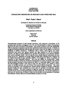
Figure 1: Example of temporal scalable video coding 1.1.2 DVC and DISCOVER interpolation algorithm In this section we describe one of the most popular frameworks for DVC, the Stanford codec [1]. In this codec, the video stream is split into Key Frames (KFs) and WynerZiv Frames (WZFs). Borrowing the terminology from the predictive video coding context, a KF and all the following WZFs before the next KF are said to form a group of pictures (GOP). Hence the distance between two successive KFs is called GOP size. The KFs are INTRA coded (i.e. without motion estimation and compensation). The Wyner-Ziv Frames are fed into a systematic channel coder. The systematic part is discarded and the parity bits are sent to the decoder. At the decoder side, an estimation of the Wyner-Ziv Frame is needed. It can be obtained by interpolation of the already decoded frames. This estimation is called Side Information (SI) and it can be considered as a noisy version of the true WZF. The channel decoder must correct these estimation errors by using the parity bits. Then, the encoding of the WZFs is completely independent from how the KFs have been encoded and decoded. The European project DISCOVER [2] implemented the Stanford architecture and defined effective tools for coding the KFs and the WZFs. It has become the reference technique for distributed monoview and multiview video coding. In this codec each WZF frame is transformed (by a 4x4-DCT) and each coefficient is quantized and divided in bit plane. The parity bits for each band for each bit plane can be generated by a LDPCA code or a turbo code. At the decoder the SI is generated by a linear motion interpolation algorithm of the closest frames available at the decoder side. The error for for each band is modelled as a Laplacian random variable and the allocation of the parity bits necessary to correct the SI is based on the variance of the Laplacian pdf. The request of parity bits are sent from the decoder to the encoder via a feedback channel. In DISCOVER the SI is generated by a linear motion interpolation algorithm of the closest frames available at the decoder side. Now, we describe into details the motion interpolation technique performed by DISCOVER. For the sake of simplicity, the GOP size (the distance between two KFs) is supposed to be equal to 2. Then, the frames

2D final

D3.4

Efficient progressive representation via Wyner-Ziv coding

7

Vectors Backward KF

Low pass Filter

u Forward Motion Estimation

v

Bidirectional Motion Estimation

Low pass Filter

w

Refinement and Smoothing

Bidirectional Motion Compensation

Images Side Information

Forward KF

Figure 2: Example of temporal scalable video coding which are interpolated are the two adjacent KFs1 . Let It−1 and It+1 be two consecutive KFs and let It be the WZF that needs to be estimated. DISCOVER MCTI consists in the following steps (see also Fig. 2): 1. Low pass filter. The two frames It−1 and It+1 are low-pass filtered, in order to smooth out noise. 2. Forward motion estimation. performed.

A motion estimation from It+1 to It−1 is

3. Motion vector splitting. For each block of the frame t centered in a generic point p, Btp , the vector that intersects the frame t in the point closest to p is searched. Then, this vector is split into u = v/2 and w = −v/2 and afterwards centered in p. 4. Bidirectional motion estimation. The vectors u and w are refined by adding to them a small variation minimizing the WMAD between blocks in It−1 and It+1 . 5. Vector median filtering. In order to avoid spatial incoherences, a weighted median filter is applied to the two motion vector fields. The SI is finally obtained as average of the motion compensated backward and forward references. This technique can be easily extended in the view domain for distributed multiview video coding. In a previous work [13], it has also been proposed to use four frames for the MCTI in order to use an high order motion interpolation (HOMI). This algorithm improves the RD performance of the linear MCTI algorithm, in particular for modelling no linear object trajectories. 1.1.3 Scalable DVC One of the drawbacks of SVC is that each layer depends strictly from the previous ones. With DVC, the different layers can be encoded and decoded independently. 1 This

is not necessarily true if the GOP size is greater than 2. In general, the two frames closest to WZF, available at the decoder side, are interpolated.

2D final

D3.4

Efficient progressive representation via Wyner-Ziv coding

8

This means that the base layer can be encoded with any technique without affecting the decoding of the WZFs. In particular, the temporal scalability is intrinsic in DVC. Indeed, the procedure of encoding and decoding for GOP sizes larger than two is very similar to the structure of hierarchical B-frames of H.264/AVC. Let us consider a GOP size equal to 4. Then, let Ik−2 and Ik+2 be two consecutive KFs. These frames are used for the estimation of the WZF at instant k. Once this frame has been decoded, the frame Ik is available at the decoder side. It can be used along with the KFs for obtaining the estimation of the WZFs at the instants k − 1 and k + 1. Tagliasacchi et al. [17] proposed a temporal scalable DVC for the PRISM codec. In this scheme the base layer has been obtained by H.263+/INTRA. The enhancement layer had been obtained by using algorithms for linear motion interpolation. In [9] and [6] a comparison of temporal scalable DVC w.r.t H.264/AVC has been performed. Moreover, for DVC coding they used an overlapped block motion compensation based side information generation module and an adaptive virtual channel noise model module. They obtained that the RD performance of scalable DVC improves the performance of H.264/INTRA but does not surpass the RD of SVC. Then, they suggest to use DVC only if there are some constraints in terms of complexity and memory at the encoder side. The independence of the enhancement layer w.r.t. the base layer for DVC has been emphasized in [9] and [10]. Indeed, also if we change the anchor frames, the enhancement layers does not change for DVC. On the contrary, another enhancement layer is needed each time that the INTRA Frames of H.264/AVC are coded in a different manner. The quality scalability is also automatically obtained with DVC: the parity bits generated by the encoder are used for improving the quality of the side information. Then, the more parity bits are sent to the decoder, the better is the quality of the decoded frames. Each set of parity bits progressively improves the PSNR of the decoded WZFs. Solutions for spatial scalability have been proposed in [9] and [7]. The authors in [9] also proposes spatial scalability for DVC. Let us suppose that n is the number of enhancement layers. The base layer is composed by downsampled frames of a factor of n. The side information for the enhancer layers is produced by upsampling and bi-cubic interpolation, preceded by a Gaussian filter. This side information will be then corrected by the parity bits. They also introduce a DVC scheme that combines temporal, spatial and quality scalability. Machiavello et al. [7] also propose a scheme for spatial super-resolution in the context of distributed video coding. In [11] and [5] the temporal scalability is extended for multiview video coding. Ozbek et al. [11] suppose to have two cameras : the right view is temporally predicted and the left view is predicted from the right one. They extend this structure for multiview by supposing that only one view camera depends from itself and the other ones are predicted by this reference view. Drose et al. [5] suppose that only a central camera is coded independently of the other ones. The temporal stream is coded with a certain GOP structure. In the position of the I frames, the frames of the other cameras are P-frames depending on the frames of the central camera, as the view progressive architecture of H.264/MVC [20]. The other frames are coded only by exploiting temporal correlation.

2D final

D3.4

Efficient progressive representation via Wyner-Ziv coding Key View

BL

Key View

WZ Views

Layer 2

Layer 1

9

Layer 2

BL

Figure 3: Example of multiview SVC with V = 4

1.2 System performance analysis Let us consider now the works of [9] and [6]: we perform here a performance analysis of DISCOVER w.r.t. some relevant video coding standards: H.264/AVC, H.264/AVC with a low complexity profile, the emerging HEVC. The low-complexity profile of H.264/AVC is obtained by switching off the rate distortion optimization. In our use-case, we have to send the different bit streams of the different standards. If a user having the BL of H.264/AVC cannot decode the B-frames encoded with HEVC and viceversa. For these reasons, it is necessary to send the EL bitstreams of H.264/AVC and HEVC. But if we suppose that all the users have a DVC decoder, the enhancement layers can be coded with a Wyner-Ziv codec, and thus one bitstream is sufficient for all the users. We have extended the temporal scalable video coding along the view axis in multiview video. We suppose that we have K cameras. One camera out of V is a Key camera. The other ones are Wyner-Ziv cameras. The base layer consists of sending only the Key views. The other views are hierarchical encoded, as in the temporal domain, as depicted in Fig. 3. Let us suppose that one out of four cameras is a Key camera and let 0 and 4 be two of these cameras. Then, in the first enhancement layer, the view number 2 is sent and for the second layer the cameras 1

2D final

D3.4

Efficient progressive representation via Wyner-Ziv coding

10

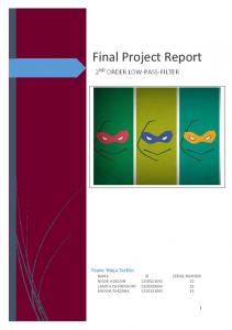
and 3 are sent. This structure is used both for the DVC codec and for H.264/MVC. If the DVC DISCOVER is not used, in order to take into account that some users can not have the H.264/MVC decoder, we are forced to encode and store also a simulcast version of this video, where each camera is independently coded. For this reasons, the performance of scalable multiview distributed video coding are compared w.r.t. H.264/MVC and H.264/Simulcast. In order to perform a complete analysis of the different methods for scalable video coding, we suppose that we have two scenarios. In the first scenario, the users have different decoders: we suppose that each video stored on the video server is coded in H.264/AVC, H.264/AVC low-complexity (with no RD optimization) and HEVC. Even if the base layers 1 and 2 are compatible, the corresponding enhancement layers will not be, since they are predicted w.r.t. possibly different images. In this context we are then obliged to send all the base layers and all the enhancement layers. Another scenario is that only the base layer is INTRA coded with H.264/AVC or HEVC, and the enhancement layers are encoded with the DISCOVER DVC scheme. These means that the enhancement layers are independent from the base layer available for each user. For the scalable monoview we have considered the MPEG sequences party scene and BQSquare, respectively at spatial resolutions of 832 × 480 and 416 × 240. Their frame rates are of 60 fps and 50 fps respectively. We have considered a GOP size of 4, and then we can suppose that we have a base layer and two enhancement layers. The frame rate for the base layer is respectively 12.5 fps and 15 fps. We have then considered DISCOVER with the base layer (that means the KFs) encoded with H.264/AVC, with HEVC and H.264/AVC (low complexity). We have performed a rate-distortion analysis of DVC w.r.t. the scenario where we are obliged to send H.264/AVC, HEVC and H.264/AVC low complexity (see Tab. 1) and we have obtained up to 23.58% of bit reduction and up to 3.54 dB of PSNR improvement. Indeed, when standard video techniques are used for the enhancement layers, we are obliged to encoded these layers with all the considered standard. With DVC, since the enhancement layers are independent of the BL, we can use the same set of parity bits independently of which BL is available to the user. In the context of multiview video coding, we have considered the Xmas sequence at 480 × 640 spatial resolution and we have compared the RD performance of DVC w.r.t. Simulcast+H.264/MVC (see Fig. 8 and 9). Indeed, if some users have not the H.264/MVC codec, we are forced to send on the net also the Simulcast version, where all the views are independently encoded.

1.3 Conclusions In this section we have performed an analysis in terms of RD performance for temporal scalable DVC w.r.t. classical scalable techniques. In contrast with the classical case, enhancement layers in DVC are independent from the BL. Then, using DVC and supposing that different users have different decoders, the same parity bits will be sufficient to decode the enhancement layers independently of the base layer codec, thus achieving a noticeable bandwidth saving. We have extended our analysis also to multiview video coding, in order to take into account that some users can have

2D final

D3.4

Efficient progressive representation via Wyner-Ziv coding

11

33

32

average PSNR [dB]

31

30

29

28

27

DISCOVER/DVC H.264 DISCOVER/DVC H.265 H264/AVC + H.264/AVC l.c. + HEVC

26

25 0.5

1

1.5

2

rate [bits/pictures]

2.5

3

3.5 5

x 10

Figure 4: RD curves for sequence Party Scene - Layer 1 - frame rate = 25 the H.264/MVC codec and others may not have it. Then, we should send also the Simulcast version of this video. If DVC is used, we can avoid to send these two versions.

2D final

D3.4

Efficient progressive representation via Wyner-Ziv coding

12

32

31

average PSNR [dB]

30

29

28

27

DISCOVER/DVC H.264 DISCOVER/DVC H.265 H264/AVC + H.264/AVC l.c. + HEVC

26

25 0.2

0.4

0.6

0.8

1

1.2

1.4

1.6

1.8

rate [bits/pictures]

2 5

x 10

Figure 5: RD curves for sequence Party Scene - Layer 2 - frame rate = 50

34

33

average PSNR [dB]

32

31

30

29

28

DISCOVER/DVC H.264 DISCOVER/DVC H.265 H264/AVC + H.264/AVC l.c. + HEVC

27

26 0.5

1

1.5

2

2.5

3

rate [bits/pictures]

3.5

4

4.5

5 4

x 10

Figure 6: RD curves for sequence BQ Square - Layer 1 - frame rate = 30

2D final

D3.4

Efficient progressive representation via Wyner-Ziv coding

13

33

average PSNR [dB]

32

31

30

29

DISCOVER/DVC H.264 DISCOVER/DVC H.265 H264/AVC + H.264/AVC l.c. + HEVC

28

27

0

0.5

1

1.5

2

2.5

rate [bits/pictures]

4

x 10

Figure 7: RD curves for sequence BQ Square - Layer 2 - frame rate = 60 40

DVC − DISCOVER H.264/MVC + H.264/simulcast

39

38

PSNR [dB]

37

36

35

34

33

32 10

20

30

40

50

60

70

rate [bits/view/picture]

Figure 8: RD curves for sequence Xmas - Layer 1 39

DVC − DISCOVER H.264/MVC + H.264/simulcast

38

PSNR [dB]

37

36

35

34

33

32 10

20

30

40

50

60

70

rate [bits/view/picture]

Figure 9: RD curves for sequence Xmas - Layer 2

2D final

D3.4

Efficient progressive representation via Wyner-Ziv coding

method DVC (KF coded with DVC (KF coded with DVC (KF coded with DVC (KF coded with DVC (KF coded with DVC (KF coded with DVC (KF coded with DVC (KF coded with DVC (KF coded with DVC (KF coded with DVC (KF coded with DVC (KF coded with

∆R [%] BQSquare - layer 1 H.264/AVC ) -4.70 HEVC ) -23.58 H.264/AVC l.c.) -4.73 BQSquare - layer 2 H.264/AVC ) 19.17 HEVC ) 4.24 H.264/AVC l.c. ) 20.20 Party Scene - layer 1 H.264/AVC ) -12.79 HEVC ) -16.36 H.264/AVC l.c.) -11.56 Party Scene - layer 2 H.264/AVC ) -13.71 HEVC ) -18.22 H.264/AVC l.c. ) -12.89

14

∆P SNR [dB] 0.86 0.40 0.20 3.54 0.83 0.84 0.80 1.07 0.78 1.06 1.08 1.02

Table 1: RD performance by Bjontegaard metric w.r.t. H.264+HEVC+H.264(lowcomplexity)

2D final

D3.4

Enhanced Intra prediction using template matching

15

2 Enhanced Intra prediction using template matching Intra prediction within H264/AVC or the current video standardization project HEVC relies on tools which are efficient when blocks to be predicted have regular or oriented textures. However, blocks which have more complex textures or have constant or smooth changing directional structures are less well predicted in this way. This is especially the case with screen content videos which contain texts, characters and non-natural elements. Template matching approaches tackle this problem in exploiting correlations between parts of pictures instead of just using pixels surrounding blocks to be predicted. After a brief reminder about prediction based on template matching, this section presents an enhancement of these methods by using weighted template matching predictors (WTM) and, then, the results once integrated in HM 4.0, the test model of HEVC.

2.1 Prediction and template matching In template matching approaches [18], intra prediction process is a 3 step method. First an area surrounding the block to be predicted, B, is defined. This is the template Y , which is often an L-shaped block (represented in Fig. 10). The second step aims at finding in the causal neighbourhood, i.e. among blocks which have already been reconstructed (see Fig. 10), pieces of picture that best matches the template. These pieces of picture are called below candidate templates Ai . Matching criteria can use metrics such as the sum of absolute differences (SAD) or mean square error (MSE) between pixels of the template Y and the candidate template Ai .

Figure 10: Search regions from causal neighbourhood. Then, N blocks Bi surrounded by the best matching areas are used to compute predictors Pi , which are then averaged to get the prediction P of the block B:

2D final

D3.4

Enhanced Intra prediction using template matching

N 1 X P = Pi N i=1

16

(1)

Intra prediction based on template matching relies on the assumption that correctly approximating the template leads to a good prediction.

2.2 Weighted template matching predictors WTM is analogous to this general approach presented above. However, it differs from it in the shapes of templates, the matching criterion and how weighting factors are computed and then used in order to get a predictor as a linear combination of template matching predictors. These differences are detailed in the following sections. 2.2.1 Shapes of template Using L-shaped templates assumes that pixels surrounding the block are as important as each other for prediction whatever the directional characteristics of the block to be predicted. WTM uses a L-shaped template also but in order to capture different texture characteristics, it takes advantage of three other templates shapes. The width and the height of respectively the right and upper parts of the L shape can be either 1 or 4 pixel large. Widths or heights of sub parts of templates are the same, whatever the size of the prediction unit (PU) for which WTM is used (4x4, 8x8, 16x16 and 32x32). The four proposed shapes are depicted on Fig. 11.

Figure 11: Shape of templates. The enlarged parts contribute more to the prediction process, which, that way, takes more into account possible directional or periodicity characteristics of the block to be predicted. The 4 shapes are separately tested in competing predictions. And once a shape is selected, a predictor P is always a linear combination of a set of predictors Pi obtained with this same template shape.

2D final

D3.4

Enhanced Intra prediction using template matching

Block B size 4x4 8x8 16x16 32x32

Table 2: Search areas characteristics Search windows number Search windows width 3 12 2 20 2 8 2 4

17

Search windows height 4 8 16 32

2.2.2 Search of templates Templates are searched in in the causal neighbourhood of the block B, as depicted in Fig. 10. However, in the HEVC context, the prediction process is related to the PU size, the PU decomposition and the prediction order of sub-blocks in the PU. In order to limit processing complexity and memory consumption, while retaining sufficient coding efficiency, the search area is not the entire causal neigbourhood but is divided into 2 or 3 rectangular and contiguous search windows. The characteristics of the search areas are summarized in Table 2. The search windows are adjacent to block to be predicted B, immediately above or on the left, as illustrated in Fig. 12. Note that this figure depicts the area scanned by the lower-right corner of the templates.

Figure 12: Search windows positions relatively to block B. These 2 or 3 windows are scanned to retain the N best candidate blocks Bi . The best candidate blocks Bi are those with the lowest Sum of square differences (SSD) between their associated template Ai and the block to be predicted template Y . The windows have been chosen small enough to keep the complexity low. However, in order to further reduce the complexity, a two-step process is adopted : • During the first step, each window is scanned on a quincunx grid starting from its upper-left corner. Therefore, the search space is sub-sampled by a factor 2. At the end of this step, N candidate blocks Bi are selected. • During the second step, for each selected block Bi , the search is refined by visiting the four neighbouring positions (left, above, right and bottom) of Bi which were

2D final

D3.4

Enhanced Intra prediction using template matching

18

not scanned during the first pass. This trade-off between performance and execution time provides almost the same performance as the classical full search, while being significantly faster. A second speed improvement is related to the shapes of templates. As these shapes overlap, it is straightforward to factorize the four searches in a single pass. 2.2.3 Computation of weights and prediction Given N candidate blocks Bi , N predictors Pi will be computed and then linearly combined as a single predictor P of the block B: P =

N X

(2)

wi Pi

i=1

where wi are the weighting factors and N is set to 3. To do so, templates (Y and Ai ) and blocks (Bi )are represented first as vectors by reading each rows to get their components. Then, each block Bi is scaled by a factor ρi in order to obtain a predictor Pi of the block B. The factor ρi is computed using the templates and the least mean squares (LMS) criterion: Ai Y ||Y ||

(3)

Pi = ρi Bi

(4)

ρi = and the predictor Pi is given by:

Finally, the predictor P of the block B is obtained by averaging the predictors Pi : P =

N 1 X Pi N i=1

(5)

1 ρi N

(6)

The initial weight wi is simply set to: wi =

In most cases, averaging several templates increases significantly the coding efficiency of template matching. However, sometimes, one or several N predictors might be so different from the block B that they impair the quality of the prediction. A threshold based strategy has been added in order to reject such outliers. The best candidate (according to the SSD metric) is always kept. The other candidates are compared to the best candidate. Those which are too far from it are rejected. All computations previously presented can be easily implemented using integer arithmetic, thanks to appropriate scaling and rounding, without loss of performance.

2D final

D3.4

Enhanced Intra prediction using template matching

Table 3: Activation of WTM according to video classes and PU sizes HE LC 4x4 8x8 16x16 32x32 64x64 4x4 8x8 16x16 32x32 Class A X X X X X Class B X X X X X X X Class C X X X X X Class D X X X X X Class E X X X X X X X Class F X X X X X X X -

19

64x64 -

Table 4: HM4.0+WTM vs HM4.0 all classes except class F All Intra HE All Intra LC Y U V Y U V Class A 0,0% -2,0% -2,6% -0,1% -1,4% -2,0% Class B -0,8% -0,9% -0,8% -0,9% -0,7% -0,6% Class C -0,9% -0,5% -0,7% -1,0% -0,6% -0,8% Class D -0,4% -0,3% -0,4% -0,5% -0,4% -0,4% Class E -0,5% -0,4% -0,4% -0,7% -0,6% -0,2% Overall -0,5% -0,8% -1,0% -0,7% -0,7% -0,8% -0,5% -0,8% -1,0% -0,7% -0,7% -0,8% ENC TIME [%] 114% 121% DEC TIME [%] 104% 105%

2.3 Experimental Results WTM has been integrated in the HM4.0. The All Intra–High efficiency (AI-HE) and All Intra–Low complexity (AI-LC) test conditions defined in [16] were used. WTM is implemented for the following sizes of prediction unit (PU): 4x4, 8x8, 16x16 and 32x32. Table 3 shows when W TM is activated (notified with an X) according to the video class and the PU size: The Results with only the classes A, B, C, D and E are presented in Table 4, while the results including class F are reported in Table 5. These results show that: • WTM always improved the intra prediction of HM4.0, • The average BD rate gains are 0.5% in HE and 0.6% in LC profiles when all classes except class F are encoded, • The average BD rate gains are 1.0% in HE and 1.1% in LC profiles when all classes are encoded (class F included). An analysis of the results per video shows that:

2D final

D3.4

Enhanced Intra prediction using template matching

20

Table 5: HM4.0+WTM vs HM4.0 all classes, class F included All Intra HE All Intra LC Y U V Y U V Class A 0,0% -2,0% -2,6% -0,1% -1,4% -2,0% Class B -0,8% -0,9% -0,8% -0,9% -0,7% -0,6% Class C -0,9% -0,5% -0,7% -1,0% -0,6% -0,8% Class D -0,4% -0,3% -0,4% -0,5% -0,4% -0,4% Class E -0,5% -0,4% -0,4% -0,7% -0,6% -0,2% Class F -3,1% -2,9% -2,8% -3,5% -3,5% -3,4% Overall -1,0% -1,2% -1,3% -1,1% -1,2% -1,2% -1,0% -1,2% -1,3% -1,1% -1,2% -1,2% ENC TIME [%] 114% 121% DEC TIME [%] 104% 105% • When only classes A, B, C, D and E are encoded, the best BD rate gains are reached for the video “basketballdrill” and are 2.4% in HE and 2.3% in LC profiles. • When all classes are encoded (class F included), the best BD rate gains are reached for the video “SlideEditing” and are 5.8% in HE and 6.5% in LC profiles.

2.4 Conclusion WTM is an intra prediction method based on weighted template matching predictors for which four different shapes of templates can be used. WTM improves intra prediction for all video classes. The average BD rate gains are 1% in HE and 1.1% LC profiles when all classes are used and 0.5% in HE and 0.6% in LC profiles also when all classes are tested except the class F. WTM performs better when videos contain non-natural content such as text, logos and scenes from video games. In these cases, average BD-rate gains are 3.1% and 3.4% in HE and LC profiles respectively.

2D final

D3.4

The “Don’t Care Region” paradigm for image and video coding

21

3 The “Don’t Care Region” paradigm for image and video coding In this section we introduce the concept of “Don’t Care Region”, that can be used for the coding of 2D and 3D video (see also D4.3). The key observation at the basis of this is that, as long as the compression error does not lead to unacceptable decoded image quality, each pixel only needs to be reconstructed coarsely at decoder, within a preestablished acceptable interval. We first formalize the notion of this tolerable range per depth pixel as don’t care region (DCR) using a threshold τ , by studying the decoded distortion sensitivity to the pixel value. This concept can be applied to images or, even more effectively, to depth images, as shown in D4.3. If a pixel’s reconstructed value is within its DCR, then the resulting distortion will stay within a range defined by a threshold τ . Given per-pixel DCRs, it is possible to modify the transform used for image compression, as shown in [4]. There, given per-pixel tolerable range for reconstruction (don’t care regions) in a code block, the sparsest transform domain representation of depth signal is sought by minimizing the l0 -norm. We have extended the approach in [4] by exploiting the degrees of freedom defined in DCRs to seek coding gain in the temporal dimension for depth video [19] . How to jointly optimize depth video in both spatial and temporal dimension given per-pixel DCR is left for future work.

2D final

D3.4

References

22

References [1] A. Aaron, R. Zhang, and B. Girod, “Wyner-Ziv coding of motion video,” in Asilomar Conference on Signals and Systems, Pacific Grove, California, Nov. 2002. [2] X. Artigas, J. Ascenso, M. Dalai, S. Klomp, D. Kubasov, and M. Ouaret, “The Discover codec: Architecture, techniques and evaluation,” in Proc. of Pict. Cod. Symp., Lisbon, Portugal, Nov. 2007. [3] Y. Chen, Y. K. Wang, K. Ugur, M. M. Hannuksela, J. Lainema, and M. Gabbouj, “The emerging MVC standard for 3D video services,” EURASIP Journal on Advances in Signal Processing, vol. 2009, 2009. [4] G. Cheung, A. Kubota, and A. Ortega, “Sparse representation of depth maps for efficient transform coding,” in IEEE Picture Coding Symposium, Nagoya, Japan, December 2010. [5] M. Drose, C. Clemens, and T. Sikora, “Extending single-view scalable video coding to multi-view based on h. 264/avc,” in Image Processing, 2006 IEEE International Conference on. IEEE, 2006, pp. 2977–2980. [6] X. Huang, A. Ukhanova, E. Belyaev, and S. Forchhammer, “Temporal scalability comparison of the h. 264/svc and distributed video codec,” in Ultra Modern Telecommunications & Workshops, 2009. ICUMT’09. International Conference on. IEEE, 2009, pp. 1–6. [7] B. Macchiavello, F. Brandi, R. Queiroz, and D. Mukherjee, “Super-resolution applied to distributed video coding with spatial scalability,” Anais do Simpsio Brasileiro de Telecomunicaes, 2008. [8] P. Merkle, A. Smolic, K. Muller, and T. Wiegand, “Multi-view video plus depth representation and coding,” in Proc. of IEEE Int. Conf. Image Proc., San Antonio, TX, 2007. [9] M. Ouaret, F. Dufaux, and T. Ebrahimi, “Codec-independent scalable distributed video coding,” in Image Processing, 2007. ICIP 2007. IEEE International Conference on, vol. 3, 16 2007-oct. 19 2007, pp. III –9 –III –12. [10] ——, “Error-resilient scalable compression based on distributed video coding,” Signal Processing: Image Communication, vol. 24, no. 6, pp. 437–451, 2009. [11] N. Ozbek and A. Tekalp, “Scalable multi-view video coding for interactive 3dtv,” in Multimedia and Expo, 2006 IEEE International Conference on. IEEE, 2006, pp. 213–216. [12] F. Pereira and T. Ebrahimi, Eds., The MPEG-4 book, ser. IMCS Press Multimedia Series. Upper Saddle River, NJ: Prentice Hall, 2002.

2D final

D3.4

References

23

[13] G. Petrazzuoli, M. Cagnazzo, and B. Pesquet-Popescu, “High order motion interpolation for side information improvement in DVC,” in Proc. of IEEE Int. Conf. Acoust., Speech and Sign. Proc., Dallas, TX, 2010. [14] H. Schwarz, D. Marpe, and T. Wiegand, “Overview of the scalable video coding extension of the H.264/AVC standard,” IEEE Trans. Circuits Syst. Video Technol., vol. 17, no. 9, pp. 1103–1120, Sep. 2007. [15] D. Slepian and J. K. Wolf, “Noiseless coding of correlated information sources,” IEEE Trans. Inf. Theory, vol. 19, pp. 471–480, Jul. 1973. [16] A. Tabatabai, E. Francois, K. Chono, H. Yu, J. Rajan, and L. J., “Ce6: Intra coding improvements,” Tech. Rep., July 2011. [17] M. Tagliasacchi, A. Majumdar, and K. Ramchandran, “A distributed-sourcecoding based robust spatio-temporal scalable video codec,” in Proc. Picture Coding Symposium, 2004. [18] T. Tan, C. Boon, and Y. Suzuki, “Intra prediction by averaged template matching predictors,” in CCNC, 2007. [19] G. Valenzise, G. Cheung, R. Oliveira, M. Cagnazzo, B. Pesquet-Popescu, and A. Ortega, “Motion prediction of depth video for depth-image-based rendering using don’t care regions,” in Proc. of Pict. Cod. Symp., 2012. [20] A. Vetro, T. Wiegand, and G. Sullivan, “Overview of the stereo and multiview video coding extensions of the h.264/mpeg-4 avc standard,” Proceedings of the IEEE, vol. 99, no. 4, pp. 626 –642, april 2011. [21] A. Wyner and J. Ziv, “The rate-distortion function for source coding with side information at the receiver,” IEEE Trans. Inf. Theory, vol. 22, pp. 1–11, Jan. 1976.

2D final

D3.4