World Academy of Science, Engineering and Technology 36 2007
Load Modeling for Power Flow and Transient Stability Computer Studies at BAKHTAR Network M. Sedighizadeh, and A. Rezazadeh of various classes, e.g., residential, commercial, industrial. Because this software has been disadvantage, therefore, we reprogrammed its algorithm with new properties by Delphi language and it named “LOADMOD”. This software is very user friendly that in this paper will be explained later.
Abstract—A method has been developed for preparing load models for power flow and stability. The load modeling (LOADMOD) computer software transforms data on load class mix, composition, and characteristics into the from required for commonly–used power flow and transient stability simulation programs. Typical default data have been developed for load composition and characteristics. This paper defines LOADMOD software and describes the dynamic and static load modeling techniques used in this software and results of initial testing for BAKHTAR power system.
II. LOAD MODELING PHILOSPHY Two main approaches to load model development have been considered by the electric utility industry: “measurement – based” and “component – based”. The measurement–based approach involves placing monitors at various load substations to determine the sensitivity of load active and reactive power to voltage and frequency variations [4] to be used directly or to identify parameters for more detailed load models [5]. This approach has the advantage of direct monit primarily consist of a general load model (A), CYME load model (B) and constant impedance load model (C). The response of active and reactive power for this bus following loss one of transmissions lines is shown in Fig. 11 and Fig. 12 respectively. In two figures, power is given in perunit on a 100 MVA base and voltage is given in p.u. based on nominal voltage. It was found that simplified models A and B are suitable for application in voltage stability studies; whereas model C does not capture the dynamic state change adequately giving wrong predictions on voltage stability behaviour. Owing of the true load can produce load model parameters directly in the form needed for power flow and transient stability program input. Its disadvantages include the cost of acquiring and installing the measurement equipment and the need to monitor all system loads or to extrapolate from limited measurements. The measurements must also be repeated as the load changes due to seasonal and other factors. The component–based approach [6], which was pursued in this paper, involves building up the load model from information on its constituent parts, as illustrated in Fig. 1. For these methods three sets of data are required: Load class mix data, Load composition data, Load characteristics data. The component-based approach has the advantage of not requiring system measurements and therefore being more readily put into use. Since load characteristics and load composition data should not vary widely over a particular system, they can be developed once for the entire system.
Keywords—Load Modelling, Static, Power Flow.
L
I. INTRODUCTION
OAD characteristics have long been known to have a significant effect on system performance, and transient stability results are known to be highly dependent upon the load characteristics assumed [1]. Because of the uncertainty of the actual load characteristics utilities have attempted to use characteristics that would lead to conservative designs. It has been shown, however, that there is no single load characteristic that leads to a conservative design for all system configurations [2]. It has become clear that assumptions regarding the load model can impact predicted system performance as significantly as the models chosen for excitation systems and synchronous machines, which have received greater industry attention. Several efforts have been made to develop methods for constructing improved load models [3]. One of the methods demonstrated the validity of a load modeling process based on the components that make up the load and the individual voltage and frequency characteristics of these components. In 1984, EPRI contracted with General electric, to develop production – grade computer programs and documentation that would provide an easy way for load modeling, this has been accomplished by the development of the load model synthesis (LOADSYN) computer program package, which permits the user to develop load models for his system with a minimum amount of data on the system loads, simply the mix Manuscript received October 6, 2007 Authors are with Faculty of Electrical and Computer Engineering, Shahid Beheshti University, Tehran, 1983963113, Iran (phone: +98-21-29902290; fax: +98-21-22431804; e-mail:
[email protected]).
272
World Academy of Science, Engineering and Technology 36 2007
KQF2 - frequency sensitivity coefficient for reactive compensation.
Only the load class mix data needs to be prepared for each bus or area, and updated for changes in the system load. Component – based load modeling is divided into two main groups: static and dynamic modeling. These groups are explained in following sections:
QO – initial bus load reactive power, from power flow base case.
The aggregation of the static load models involves the following steps: 1- Determine the bus load composition, i.e., the fraction of each component at a particular bus (or zone or area), by combining the load class mix and the class composition data. 2- Use the bus load composition fractions as weighting factors to compute a weighted average of the individual component sensitivity factors. IV. DYNAMIC AGGREGATION Model 1: The motor components are aggregation into a single dynamic induction motor model, using the standard equivalent circuit shown in Fig. 2.
Fig. 1 Component – based load modeling
III. STATIC AGGREGATION In developing an aggregate static model, the sensitivity factors of the individual load components are aggregated into values that can be used as exponents in the following “ general load model” : V V P = Pa1( )KPV1(1. + KPF1Δf ) + (1. − Pal)( )KPV2 PO VO VO
(1)
Fig. 2 Induction motor model
V Q V Q =Qa1( )KQV1(1. + KQF 1Δf ) +( O −Qal)( )KQV2(1. + KQF2Δf ) VO PO VO PO
(2)
The mechanical load torque is represented as the following polynomial function of motor speed: TM= TMO ( A ωm2 + Bωm +C)
The parameters in this formula are defined follows:
(3)
The acceleration of the motor is represented by:
Pal – frequency dependent fraction of active power load.
ωm = 1/2H [ TM (ω) –TE(S)]
KPV1- Voltage exponent for frequency dependent active power load.
(4)
where TE is the electrical torque, which is a function of the motor slip, s. The motor is disconnected if the bus voltage stays below VT for longer than TI seconds. Motor parameters are aggregated and presented in [7].
KPV2- Voltage exponent for non-frequency dependent active
power load. KPF1 – frequency sensitivity coefficient for active power load.
Model 2: Because diversity in motors rating is very wide in industrial centers, therefore it is better for increase in accuracy of modelling, we peresent dynamic load model with two motors. The relevant equations for calculating electric parameters of the two – motor model have been developed and presentd in [7]. The motor model has been developed and presented in the flow chart of Fig. 3.
Δf – per unit frequency deviation from nominal. V – per unit voltage magnitude at the bus. VO- initial voltage magnitude from power flow base case. PO – initial bus load active power, from power flow base case. Qal – reactive load coefficient – ration of initial uncompensated reactive load total to initial active power load P0 KQV1 – Voltage exponent for the uncompensated reactive
power load. KQF1 - frequency sensitivity coefficient for uncompensated
reactive power load. KQV2 – Voltage exponent for reactive compensation term.
273
World Academy of Science, Engineering and Technology 36 2007
The user provides input to general load modeling program to describe the load on each bus or group of buses (zones, areas) by the percentage mix of load classes such as residential, commercial, industrial and power plant auxiliary, etc. Each load class is defined, in a database file, by its percentage composition in terms of components, such as window air conditioner incandescent lighting, refrigeration, etc. Default data is provided as part of the software package for this composition data. The parameters defining the voltage and frequency characteristics and dynamic characteristics of each of the load components are stored in another database file, supplied with the software package, which can be easily modified by the user to add more components or use new data that becomes available. The general load models generated by software are transferred to the special load modeling program, which generates “specific load models” in the forms required by the specific power flow and transient stability programs. When running special load modeling program, the user can also select which of the models available in the particular power flow or stability program, are to be used for certain buses or groups of buses.
Fig. 3 Flow chart for motor separation based on eigen values method
VI. LOADMOD SOFTWARE TESTING FOR BAKHTAR POWER SYSTEM
V. LOAD MODELING COMPUTER PROGRAM The load modeling program package (LOADMOD) that has been defined in this paper, has following advantages in contrast to (LOADSYN) package: 9 Common graphic user interface 9 Integrated data base editor and manager for all kinds of data 9 flexible enough to be directly applicable to utilitytype load and industrial three-phase load in electric power systems 9 compatible with windows98,2000,XP 9 Powerful mouse and ribbon-driven Pan and Zoom facilities. 9 data available and/or entered in tabular form 9 access to graphical reporting facilities 9 Tabular or Dialog Data Entry 9 The outline, contents and units of the generated tabular reports are completely user defined 9 Graphical visualization of results by labeling components with a simple mouse action 9 User-Defined Graphical Reports 9 Copy and Paste through clipboard 9 Representation of dynamic load model with double cage induction motor for rise precision
The LOADMOD was tested by BAKHTAR power system network. This network has several buses load (63/20 kv). In this paper all of the buses modeled with LOADMOD. Routine for this modeling is explained in following: A. Preparing Load Class Mix Data for BAKHTAR Power System Load class mix data is the percentage fractional composition of the bus load by load classes. This shows the percentage of each residential, commercial or industrial loads for the sampled bus bar. Load class mix data is different for each and every bus and it is changing with weather and other climatic conditions of the region. These data are normally not available or is very difficult to set up in a large scale power system. Different methods are presented for collecting these data and classification of the system loads. The method explained in this paper is collecting these data from customer billing data, which includes the energy consumption of every costumed for two months period. Power system companies are usually having different pricing protocol for each consumer according to its use. Load class mix data is as input data for software, but for BAKHTAR power system is as a default in software. B. Load Class Mix Data for Each Region The BAKHTAR power system network is divided into several regions that a part of them as presented by Table I. Form the two months customer billing information available from load forecasting department, the customer energy consumption (MWh) is categorized to industrial, utilities, commercial and residential. The results shown in Table I present the percentage energy consumption of the total load in
The load modeling program package (LOADMOD) converts load mix, load composition, and load characteristic data into the parameters required for power flow and transient stability programs. LOADMOD is composed of on input data file, two programs and two data bases. These programs and databases are including: Load characteristic data base, load composition data base, general load modeling program and special load modeling program.
274
World Academy of Science, Engineering and Technology 36 2007
TABLE II A PART OF LOAD CLASS MIX DATA FOR OVER DISTRIBUTION SUBSTATIONS OF BAKHTAR POWER SYSTEM FOR THE MONTHS OF MAY AND JUNE 2005 Resi Agr. Ind Com. Lig Bus name
each region and for the province as a whole, for the months of May and June 2005. This table is repeated for the six two months of the year to obtain the variations of the load mixture over the year. With some approximation the Table I can be used to have modeling for the first six months of the year and also data for two months of October and November 2005 can be used to have load modeling for the second six months of the year.
Bahar Mrianj Laljin AsadAbad KabodrAhang Sarkan Jokar Gahavand Khazal Gorveh Shisheh SimanHegmatan SimanEkbatan
C. Load Class Mix Data for Each Bus In the second level of classification each region is broken further into three parts: municipality, industrial and district as each one of them is called a zone. In every power system network, the total numbers of zones are equivalent to number of regions into three. Load class mix data for each zone is found out similar to that of each region. Classification is followed here to obtain load mixtures for these new subsections with in each region. Infact, the above classification divides the system into 78 zones with associated defined characteristics [7]. For the 78 segments of the BAKHTAR power system (municipality, industrial and district), characteristics were derived containing the load mixture for the whole year. This information was stored in data base for the Production of load mix in base cases for different times of the year .For the BAKHTAR power system all over – distribution substations (63/20 kV) are considered to be a bus bar.
(%)
(%)
(%)
(%)
(%)
32.92 39.70 75.36 32.13 32.12 85.04 90.30 68.63 25.45 84.18 0.00 0.00 0.00
30.45 8.89 0.00 50.63 43.80 0.02 0.06 15.11 63.60 0.00 0.00 0.00 0.00
24.10 33.27 0.45 2.73 6.87 1.13 0.34 4.52 2.66 1.18 100. 100.0 100.0
5.88 10.96 16.86 8.33 11.08 6.57 3.56 5.99 2.79 7.42 0.00 0.00 0.00
6.65 7.18 7.32 6.17 6.13 7.24 5.75 5.75 5.50 7.22 0.00 0.00 0.00
Load class mix data is as input for software but this data for BAKHTAR power system is as a default in LOADMOD. Menu
for input data is shown in Fig. 4.
TABLE I A PART OF LOAD CLASS MIX DATA FOR AREA OF BAKHTAR POWER SYSTEM FOR THE MONTHS OF MAY AND JUNE 2005 Resi Agr. Ind Com. Lig Area name
Arak Delijan Saveh Farahan Hamadan Malayer Toyserkan Razan Nahavand Gorveh
(%)
(%)
(%)
46.00 24.07 19.71 32.61 52.73 41.34 50.54 23.03 46.06 84.18
13.43 2.28 11.90 29.54 9.97 30.49 21.89 28.08 29.95 0.00
20.31 60.81 55.84 12.97 15.04 10.97 8.92 33.61 5.57 1.18
(%) 13.63 7.53 5.93 5.41 14.21 10.44 12.32 4.64 12.65 7.42
(%) 6.63 5.31 6.61 19.47 8.06 6.76 6.34 10.63 5.77 7.22
Fig. 4 Menu for load class mix input data
D. Load Composition Data Base These data are infact showing percentage of the load composition such as refrigerator, air conditioning, lighting and etc, for a total load class mix in each every bus bar. Load composition data can very significantly with time of day, day of week, season, and weather. However, it may be find for four or two seasons of the year like winter and summer. It may also be prudent in some studies to assume the same load model for each season in a power system network .For a typical power system network these data are not too much variable and can be counted as a bus bar in that network for load modeling . These data are same from one bus bar to the other. In warm climates, summer load may include large amounts of air conditioning load .Winter Loads may consist of electric heating in areas of low energy cost, or heat pump in other areas. Both air conditioning and heating loads are seasonal, but are also very sensitive to weather .Cold, windy weather will increase heating load and hot, humid weather will increase air conditioning load. Weekday load is likely to be
Load class mix data for each bus bar can be known simply by knowing the bus bar location in the region and zone. Table II shows a part of load class mix data for over-distribution substations (bus bar) of the BAKHTAR power system for the months of May and June 2005. The kind of substation voltage and capacity of the over – distribution substations of the BAKHTAR power system are known and easily available with load forecasting department.
275
World Academy of Science, Engineering and Technology 36 2007
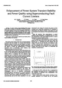
VII. LOAD MODEL SIMULATION
dominated by industrial loads. Up to 90% of the load in some industrial plants is motor load. Commercial building loads are largely consists of air conditioning and discharge lighting. Agricultural load are largely consists of motors driving pumps, especially in growing seasons. Composition data defaults for LOADMOD are 18 cases of US and 2 cases for BAKHTAR power system as shown in Table III. This data base can be developed by user. Menu for load composition data is shown in Fig. 5.
In this paper simulations made at MALAYER1 substation of BAKHTAR power system to determine the sensitivity of the load to voltage and frequency changes. Figs. 9 and 10 show the results of one of these simulations. Different load configuration is studied. The simplified load used as a reference on MALAYER1 substation primarily consist of a general load model (A) ,CYME load model (B) and constant impedance load model (C). The response of active and reactive power for this bus following loss one of transmissions lines is shown in Fig. 11 and Fig. 12 respectively. In two figures, power is given in perunit on a 100 MVA base and voltage is given in p.u. based on nominal voltage. It was found that simplified models A and B are suitable for application in voltage stability studies, whereas model C does not capture the dynamic state change adequately giving wrong predictions on voltage stability behaviour.
E. Load Characteristics Data This data is third sets of data required for modeling. These are a set of parameters such as power factor, variation of power with voltage, etc., that characterize the behavior of a specified load. They can be of either static model or dynamic model these characteristics can be obtained for each load component during the laboratory of factory tests. To obtain load characteristics data for BAKHTAR power system, 29 components mentioned in Table III are to be tested which is a very difficult task due to numbers of them. The results of laboratory experiments on six of them such as air conditioning (CRAR, PRAR), refrigerator (REFR), cloth washer (CWSH), color television (TVSN), water heater (ELWH) and florescent lights (FLIT) are presented in [7]. Static and dynamic load component are found out as explained in [8,9]. To find out N m we divided total motor power of the component to the consumption power of the component. Table IV presents static and dynamic characteristics of the components which have been used. However, it would have been much better if all 29 components would have been tested and their characteristics are modeled. Table IV is as a data base for load mod software. A part of this data base is shown in Fig. 6.
Fig. 5 Menu for load composition data
F. General Modeling Program Static general modeling option in main menu software creates general load models as described in (1), (2) equations, from data on mix, composition and characteristic. Typically for BAKHTAR power system, static modeling is shown in Table V. A part of output data for static general model is shown in Fig. 7. Software outputs for dynamic modeling (single and two induction motor) are shown in Table VI, VII.
TABLE III LOAD COMPOSITION DATA FOR BAKHTAR POWER SYSTEM Equipment Code class Winter(%) Summer(% )
G. Special Modeling Program This program transforms the general load models in to the specific formats and detail levels required by several common-used power flow and transient Stability programs – namely, the EPRI [10], CYME Company [10], and power technologies, Inc (PTI) [10] programs. Interface to other programs can be easily added. Typically BAKHTAR power system is shown in Table VI. A part of output data for static special model is shown in Fig. 8.
276
Electric heater
REHT
Residential
6
43
Pump heater
RSPM
Residential
0
0
Pump aircon.
RCPM
Residential
0
0
Central aircond.
RCAR
Residential
0
0
Room aircond.
RRAR
Residential
0
27.6
Elec. Water heat.
ELWH
Residential
0
0
range
ELRA
Residential
0
0
Refrigrator
REFR
Residential
49.5
35.9
Dish washer
DWSH
Residential
0
0
Cloth washer
CWSH
Residential
1.3
1
Cloth dryer
DRYR
Residential
0
0
Lighting
ILIT
Residential
38.4
37.8
Television
TVSN
Residential
10
7.2
Floor fan
FFAN
Residential
0
0
Pump heater
CSPM
Commercial
4.4
0
World Academy of Science, Engineering and Technology 36 2007
Pump aircon.
CCPM
Commercial
0
0
Central aircond.
CCAR
Commercial
0
0
Room aircond.
CRAR
Commercial
0
30
Florecent ligh.
FLIT
Commercial
47.7
35.5
Other light.
ILIT
Commercial
47.7
47.7
Alum. Electrolis.
ELTR
Industrial
100
100
Iron.arc furn.
FURN
Steel indu.
25
25
Iron small drives
SINM
Steel indu.
35
35
Iron large drives
LINM
Steel indu.
40
40
Other small drives
SMOT
Industrial
65
65
Other large drives
LMOT
Industrial
35
35
Agricul. Water pump
AGMP
Agricultral
100
100
Power plant auxiliaries
PPAU
Power plant
100
100
Fig. 7 Menu for general load model data TABLE V A PART OF GENERAL LOAD MODEL FOR BAKHTAR POWER SYSTEM Malayer1
AsadAbad
Hamedan
HosseinAbad
SalehAbad
P0
26.7
29.2
30.1
11.3
16.0
Q0
12.9
14.1
14.6
5.5
7.7
KPV1
0.96
1.17
0.78
0.94
1.17
KPV2
1.42
1.42
1.42
1.45
1.42
KQV1
0.7
2.08
-1.18
1.76
2.08
KQV2
2
2
2
2
2
KPF1
2.79
3.73
1.61
3.69
3.73
KQF1
1.95
1.84
2.24
1.49
1.84
KQF2
1
1
1
1
1
Pa1
0.84
0.87
0.78
0.92
0.87
Pa2
0.16
0.13
0.22
.08
0.13
Qa1
0.44
0.48
0.38
0.51
0.48
Qa2
0.56
0.52
0.62
0.49
0.52
Fig. 6 Menu for load characteristics data
TABLE IV LOAD CHARACTERISTICS DATA FOR BAKHTAR POWER SYSTEM
277
World Academy of Science, Engineering and Technology 36 2007
TABLE VI ESTIMATED VALUES OF A SINGLE MOTOR MODEL
TABLE VIII A PART OF SPECIAL LOAD MODEL FOR BAKHTAR POWER SYSTEM
Malayer1
AsadAbad
Hamedan
HosseinAbad
SalehAbad
Malayer1
AsadAbad
Hamedan
HosseinAbad
SalehAbad
P0
26.7
29.2
30.1
11.3
16.0
P0
26.7
29.2
30.1
11.3
16.0
Q0
12.9
14.1
14.6
5.5
7.7
Q0
12.9
14.1
14.6
5.5
7.7
Rs
0.04
0.04
0.05
0.03
0.04
P1
0.52
0.6
0.46
0.49
0.6
Xs
0.1
0.09
0.1
0.09
0.09
P2
0
0
0
0
0
Rr
0.04
0.04
0.05
0.03
0.04
P3
0.48
0.4
0.54
0.51
.4
Xr
0.11
0.12
0.1
0.14
0.12
Q1
1.43
2.04
0.8
1.88
2.04
Xm
2.58
2.71
2.38
2.91
2.71
Q2
0
0
0
0
0
h
0.59
0.64
0.51
0.73
0.64
Q3
-0.43
-1.04
.20
-0.88
-1.04
A
0.65
0.74
0.51
0.84
0.74
LDP
0
0
0
0
0
LDQ
0
0
0
0
0
B
0
0
0
0
0
TABLE VII ESTIMATED VALUES OF A TWO MOTOR MODEL Malayer1
AsadAbad
Hamedan
HosseinAbad
SalehAbad
P0
26.7
29.2
30.1
11.3
16.0
Q0
12.9
14.1
14.6
5.5
7.7
Rs
0.04
0.04
0.03
0.02
0.06
0.09
0.05
0.11
0.06
0.11
0.12
.10
0.13
0.10
0.12
0.12
0.13
0.14
0.13
0.15
0.03
0.05
0.06
0.03
0.02
0.07
0.06
0.12
0.05
0.09
0.132
0.14
0.13
0.18
0.16
0.135
0.16
0.12
0.17
0.13
2.95
3.27
2.44
3.76
3.7
2.56
3.18
2.54
3.27
3.5
0.82
0.92
0.56
0.67
0.55
1.50
1.65
1.11
1.81
1.13
Xs
Rr
Xr
Xm
Fig. 8 Menu for special load model data
1.4 1.3
real power(pu)
1.2
h
1.1 1 0.9
A
0.81
0.91
0.61
0.94
0.44
1.55
1.65
1.18
1.75
1.25
0
0
0
0
0
0.8 0.7 1.06 1.04
1.3
1.02
B
1.2
1
1.1 0.98
1 0.96
0
0
0
0
0
frequency(pu)
0.9 0.94
0.8 voltage(pu)
Fig. 9 Sensitivity of the active power to voltage and frequency changes for MALAYER1 substation
278
World Academy of Science, Engineering and Technology 36 2007
VIII. CONCLUSION The load modeling (LOADMOD) software has been designed to use, to the fullest extent possible , the present load modeling capabilities in commonly – used power flow and stability programs. The LOADMOD programs with their associated documentation and default data bases provide the electric utility industry with an easy way to begin immediately to obtain improved load models for power flow and stability analysis. Yet they also provide a flexible framework for incorporating improved data and models as these are developed.
1.4 1.3
reactive power(pu)
1.2 1.1 1 0.9 0.8 0.7 1.06 1.04
1.3
1.02
1.2
1
1.1 0.98
1 0.96
0.9 0.94
frequency(pu)
0.8 voltage(pu)
REFERENCES
Fig. 10 Sensitivity of the reactive power to voltage and frequency changes for MALAYER1 substation
[1]
IEEE Task Force on load representation for dynamic performance. Bibliography on load models for power flow and dynamic Performance Simulation: .IEEE Trans. On power Systems. Vol. 10. No.1 .1995. [2] O. Ruhle, Instructions for Data input to NETOMAC. Siemens AG, 1996. [3] R. Balanathan, N. C. Pahaolawaththta and U. D. Annakkage. Undervoltage Load shedding for induction Motor dominant loads considering P.Q Coupling. IEE Proc – Gener. Transm Distr. Vl .146, No.4 July. [4] A. Borghetti, R. Caldon. A. Mari and C. Nucci, On Dynamic Load Models for voltage stability studies .IEEE Trans. Power systems Vol.12, No.1 .Feb.1993. [5] D.J.Hill .Nonlinear Dynamic Load Models with Recovery for voltage stability studies. IEEE Trans. Power Systems Vol.8 .No.1. Feb.1993 [6] D. Karlsson and D. J. Hill. Modeling and identification of Nonlinear Dynamic Loads in power systems. IEEE Trans. Power Systems, Vol.9 No.1, Feb.1994. [7] M. Sedighizadeh, M. Kalantar load modeling with component based methods, M. S. thesis , IUST, Nov 1998 [8] G. Rogers, J. di Manno and R. Alden, An Aggregate induction Motor model for industrial Plants. IEEE Trans. On PAS, No.4, 1984. [9] F. Nozari, M. Kankam, W. Price. Aggreagation of induction motors for transient stability Load modeling. IEEE Trans. on power Systems. Vol.2 1987. [10] M. Taleb, M. Akbaba and E. Abdullah, Aggregation of induction machines for power System Dynamic Studies., IEEE Trans. On Power Systems. Vol. 9 .1994.
1.005 Model B
Active Power(pu)
1
Model A 0.995 Model C
0.99
0.985
0
2
4
6
8
10 12 time( sec)
14
16
18
20
Fig. 11 Transient load responses, active power for MALAYER1 bus
0.81 Model B
M. Sedighizadeh received the B.S. degree in Electrical Engineering from the Shahid Chamran University of Ahvaz, Iran and M.S. and Ph.D. degrees in Electrical Engineering from the Iran University of Science and Technology, Tehran, Iran, in 1996, 1998 and 2004, respectively. From 2000 to 2007 he was with power system studies group of Moshanir Company, Tehran, Iran. Currently, he is an Assistant Professor in the Faculty of Electrical and Computer Engineering, Shahid Beheshti University, Tehran, Iran. His research interests are Power system control and modeling, FACTS devices and Distributed Generation.
0.8
Reactive Power(pu)
0.79 Model C
0.78 Model A 0.77 0.76 0.75 0.74 0.73
0
2
4
6
8
10 12 time( sec)
14
16
18
A. Rezazade was born in Tehran, Iran in 1969. He received his B.Sc and M.Sc. degrees and Ph.D. from Tehran University in 1991, 1993, and 2000, respectively, all in electrical engineering. He has two years of research in Electrical Machines and Drives laboratory of Wuppertal University, Germany, with the DAAD scholarship during his Ph.D. and Since 2000 he was the head of CNC EDM Wirecut machine research and manufacturing center in Pishraneh company. His research interests include application of computer controlled AC motors and EDM CNC machines and computer controlled switching power supplies. Dr. Rezazade currently is an assistant professor in the Power Engineering Faculty of Shahid Beheshti University.
20
Fig. 12 Transient load responses, active power for Malayer1 bus
279