Jan 13, 2017 - Syengo Charles Kilunda (PAUISTI). Thesis Defense. Jan 13, 2017. 1 / 32 ..... Sine: m2(x) = 2 + sin(2Ïx). Syengo Charles Kilunda (PAUISTI).
Local Polynomial Regression Estimator of the Finite Population Total under Stratified Random Sampling: A Model-Based Approach Syengo Charles Kilunda Supervised by: 1. Prof. R. Odhiambo 2. Dr. G. Orwa MS300-0006/2015
Jan 13, 2017
Syengo Charles Kilunda (PAUISTI)
Thesis Defense
Jan 13, 2017
1 / 32
Overview 1
Introduction Background Information Problem Statement Objectives of the Study Main Objective Specific Objectives
2 3
Literature Review Methodology Introduction Local Polynomial Regression Estimation of the unknown function m(.)
The Proposed Estimator Properties of the Proposed Estimator ˆLP is Asymptotically Model-Unbiased Y ˆLP Mean Square Error (MSE) of Y 4
5
Simulation Study Description of population Performance Criteria Results Discussion
Syengo Charles Kilunda (PAUISTI)
Thesis Defense
Jan 13, 2017
2 / 32
Introduction
Background Information
Background Information
In sample surveys, the objective is to obtain information about the population, then use this information to make inference about some population quantities. Such information can be collected by either sampling methods or census. In sample surveys, can use auxiliary information at the estimation stage of finite population quantities (totals or mean) to increase precision of estimators of such finite population quantities (Dorfman, 1992). With availability of auxiliary information, nonparametric regression may be used in estimation of finite population totals or means. Nonparametric-based estimation is often more robust and more flexible than inference based on parametric regression models or design probabilities (i.e. design-based inference) (Dorfman, 1992).
Syengo Charles Kilunda (PAUISTI)
Thesis Defense
Jan 13, 2017
3 / 32
Introduction
Background Information
Background Information Ctd... Approaches to construction of more efficient estimators:- Model-based and design-based methods. - Model-based approach :- The regression model of y on x is used to predict the non-sampled y 0 s and, consequently their total (or other functions of interest). - Design-based approach :- Here, the probability structure of the procedure by which the sample s is selected serves as the basis for inference. Advantages: Model-based estimators generally ignore sampling probabilities. It also ignores stratum boundaries and also an automatic estimator. In this thesis, focus is on ”Model-based approach” which is based on superpopulation models ξ.
Syengo Charles Kilunda (PAUISTI)
Thesis Defense
Jan 13, 2017
4 / 32
Introduction
Problem Statement
Problem statement Over years, scientists have used auxiliary information on a character x to estimate the finite population total or mean of character y under study ´ (e.g. Montanari and Ranalli 2003, 2005; Sanchez-Borrego and Rueda 2009; Rady and Ziedan 2014b,a; Orwa et al. 2010). Most scientists have used estimators based on simple random sampling to estimate population totals Y in a model-based approach in the case of local polynomial regression. From the literature review, no work has been found concerning the development of model-based local polynomial regression estimators of a finite population total Y under stratified random sampling. Recent works by Orwa et al. (2010) and Ngesa et al. (2012) have shown that estimators developed under stratified sampling are better than those based on simple random sampling. Hence need for this particular study.
Syengo Charles Kilunda (PAUISTI)
Thesis Defense
Jan 13, 2017
5 / 32
Introduction
Objectives of the Study
Main Objective
To determine and investigate the theoretical properties of a local polynomial regression estimator of the finite population total under stratified random sampling in a model-based approach.
Syengo Charles Kilunda (PAUISTI)
Thesis Defense
Jan 13, 2017
6 / 32
Introduction
Objectives of the Study
Specific Objectives
1
To determine a model-based estimator of the finite population total using local polynomial regression under stratified random sampling.
2
To investigate the asymptotic properties (asymptotic model unbiasedness and consistency) of the proposed estimator.
3
To conduct a simulation study to compare the performance of the proposed estimator against existing ones namely Horvitz-Thompson estimator, the Linear regression estimator (Cochran, 1977, p. 200), and the Mixed ratio estimator of Orwa et al. (2010).
Syengo Charles Kilunda (PAUISTI)
Thesis Defense
Jan 13, 2017
7 / 32
Literature Review
Literature Review Neyman (1938) work thought as the first attempt to use auxiliary information Cochran (1940), in developing a ratio estimator, also used auxiliary information. Later, Cochran (1977) used auxiliary information to propose regression estimators under stratified random sampling. In most cases, a linear model is assumed, then employed to incorporate auxiliary information in construction of estimators. Sometimes the linear model is inappropriate, and hence the resulting estimators do not beat the purely design-based estimators. Due to this, several researchers have considered nonparametric models. E.g. Nadaraya (1964), Watson (1964), Dorfman (1992) and Chambers et al. (1993) who introduced model-based nonparametric kernel regression estimators. In model-based approach, the model ξ is used to predict the non-sampled values ¯ or total Y . of the population, and hence the population quantities mean Y Breidt and Opsomer (2000) considered nonparametric models within a model-assisted approach and obtained a local polynomial regression estimator as a generalization of the ordinary generalized regression estimator. Syengo Charles Kilunda (PAUISTI)
Thesis Defense
Jan 13, 2017
8 / 32
Literature Review
Literature Review Ctd... ´ Sanchez-Borrego and Rueda (2009) extended Breidt and Opsomer (2000) idea and considered a general working model through a nonparametric class of models ξ within model-based approach to inference. Orwa et al. (2010) proposed a mixed ratio estimator of finite population total under stratified sampling in a model-based approach. Their estimator yields better results as compared to the usual ratio estimator, which is design-based. Their estimator is both asymptotically unbiased and consistent. Most recently, Rady and Ziedan (2014a) has developed a model-based local linear regression estimator of the finite population total in a bivariate case but under simple random sampling. Their estimator beats the classical regression estimator when the model is misspecified, a proof of robustness. In this study, focus is on the estimation of finite population total using local polynomial regression in the presence of one auxiliary variable under stratified random sampling; And this is in the context of model-based approach to inference. Syengo Charles Kilunda (PAUISTI)
Thesis Defense
Jan 13, 2017
9 / 32
Methodology
Introduction
Methodology: Introduction Suppose we have a population of N units i.e. U = 1, 2, . . . . . . ., N. Let s be a random sample of size n selected according to some sampling design, say d, with the first order inclusion probability πi . Let yi be the value of the study variable y , for the i th population element. Let also xi be the auxiliary variate which is available for all population units in U and associated to yi . We define a finite population total as follows Y =
N X i=1
X X yi = yi + yi i∈s
(1)
i∈r
where r is the non-sampled yi0 s. P P The first component yi in Equation (1) is known while the second yi i∈s
i∈r
requires prediction which is of interest in this particular study.
Syengo Charles Kilunda (PAUISTI)
Thesis Defense
Jan 13, 2017
10 / 32
Methodology
Local Polynomial Regression
Methodology: Local Polynomial Regression Various nonparametric methods exist for the prediction of the P nonsampled component yi . In this thesis, we focus on local i∈r
polynomial regression, a kernel-based technique, in the context of stratified random sampling. Let the superpopulation model describing the relationship between the survey variable yi and the auxiliary variable xi be defined as yi = m(xi ) + ei
(2)
where the unknown function m(xi ) is assumed to be a smooth function. The error terms ei0 s are assumed to be independently distributed random variables with mean 0 and variance σ 2 (x). Model (2) treats the proxy values yi0 = m(xi ) as the predicted values of the unobserved values yi , i ∈ r .
Syengo Charles Kilunda (PAUISTI)
Thesis Defense
Jan 13, 2017
11 / 32
Methodology
Local Polynomial Regression
Estimating m(.) using Local polynomial regression
Let Kb (u) = b−1 K (u/b), where K denotes a continuous kernel function and b is the bandwidth. Consider a Taylor series expansion of the unknown function m(.) i.e. 0
m(xi ) ≈ m(x0 ) + m (x0 )(xi − x0 ) + ..... + m(p) (x0 )(xi − x0 )p
1 p!
(3)
for xi in the neighbourhood of a point of interest, x0 . Note that Taylor’s theorem says that any k−times differentiable or continuous function can be approximated with a polynomial.
Syengo Charles Kilunda (PAUISTI)
Thesis Defense
Jan 13, 2017
12 / 32
Methodology
Local Polynomial Regression
Estimating m(.) using Local polynomial regression Define the local kernel weights as wi = Kb (xi − x0 ) At a target value, x0 , the local weighted sum of squares is given by n X
wi yi − β0 −
p X
2 βj (xi − x0 )
j
(4)
j=1
i=1
In this case, the estimator is ˆ 0 ) = βˆ0 m(x
(5)
�T
�
where βˆ = βˆ0 , βˆ1 , βˆ2 , ....., βˆp is the value of β = (β0 , β1 , β2 , ....., βp )T that minimizes the local weighted sum of squares in equation (4) The solution ˆ β(x) = (XsjT W Tsj Xsj )−1 X Tsj WsjT Ys exists as long as
0
Xsj Wsj0 Xsj
Syengo Charles Kilunda (PAUISTI)
(6)
is invertible.
Thesis Defense
Jan 13, 2017
13 / 32
Methodology
Local Polynomial Regression
Estimating m(.) using Local polynomial regression From Equation (6), a consistent prediction of the unknown m(.) based on the whole finite population is given by ˆ 0 ) = βˆ0 (x) = eT1 (XsjT W Tsj Xsj )−1 X Tsj WsjT Ys = wsjT Ys m(x
(7)
where e1 = (1, 0, 0, ....., 0)T is a column vector of length p + 1; Ys = [yi ]i∈s ; Wsj = diag{Kb (xi − x0 )}i∈s and Xsj = [1, (xi − x0 ), ......, (xi − x0 )p ]i∈s . Equation (7) holds as long as XsjT W Tsj Xsj is a nonsingular matrix. Consequently, the model-based local polynomial regression estimator for Y is given by X X ˆlp = ˆi Y yi + m (8) i∈s
i∈r
where r is the nonsampled set. Now the estimator in Equation (8) is extended to stratified random sampling using one auxiliary variable.
Syengo Charles Kilunda (PAUISTI)
Thesis Defense
Jan 13, 2017
14 / 32
Methodology
The Proposed Estimator
The Proposed Estimator Consider a population consisting of N units. Suppose this population is divided into H disjoint strata, each of size Nh , h = 1, 2, ...., H. Let yhj , j = 1, 2, ...., Nh be the survey measurement for the j th unit in the hth stratum. Further, let xhj , j = 1, 2, ...., Nh be the auxiliary measurement positively correlated with yhi . From each stratum, a simple random sample of size nh is selected without replacement, where nh is sufficiently large with respect to Nh and fh = nh /Nh −→ 0. Let sh be the sample in the hth stratum and rh be the nonsampled set in the hth stratum. Define the finite population total as Y =
H X
yhs +
h=1
where yhs =
nh P
yhj and yhr =
j=1 Syengo Charles Kilunda (PAUISTI)
Nh P
H X
yhr
(9)
h=1
yhj .
j=nh +1 Thesis Defense
Jan 13, 2017
15 / 32
Methodology
The Proposed Estimator
yhj0 s
Suppose the distribution generating is given by the superpopulation model, ξ in which yhj = m(xhj ) + ehj (10) where ehj0 s are independently distributed random variables with mean 0 and variance σ 2 (xhj ). Accordingly, E(yhj ) =m(xhj ) (11) ( Cov (yhj , yh0 j 0 ) =
σ 2 (xhj ), 0,
for otherwise
h = h0
and
j = j0
(12)
where σ 2 (x) and m(x) are assumed to be continuous and twice differentiable functions of x, and σ 2 (x) > 0 Adopting Equations (6), (7) and (8), a model-based local polynomial regression estimator of the nonsampled yhj0 s in the hth stratum is therefore given by � �−1 ˆ hj = e1T XhjT Whj Xhj m XhjT WhjT y = whjT y (13) where e1 = (1, 0, 0, ....., 0)T is a column vector of length p + 1; y = [yhj ]j∈s ; � � h Whj = diag {Kb (xhj − xhi )}j∈s and Xhj = 1, (xhj − xhi ) , ......, (xhj − xhi )p j∈s . h
Equation (13) holds as long as XhjT Whj Xhj is a nonsingular matrix. Syengo Charles Kilunda (PAUISTI)
Thesis Defense
h
Jan 13, 2017
16 / 32
Methodology
The Proposed Estimator
ˆLP and the Denoting the estimator for the finite population total by Y th ˆ estimator within the h stratum by YLPh . Therefore, in stratum h, the estimator of the population total based on local polynomial regression is Nh X
ˆLP = yh + Y s h
ˆ hj m
(14)
j=nh +1
and the estimator for the finite population total is Nh H H X X X ˆLP = ˆLP = yhs + ˆ hj Y Y m h h=1
with yhs =
nh P
h=1
(15)
j=nh +1
yhj .
j=1
Syengo Charles Kilunda (PAUISTI)
Thesis Defense
Jan 13, 2017
17 / 32
Methodology
Properties of the Proposed Estimator
Properties of the Proposed Estimator
Assumptions made are: (i) (ii) (iii) (iv)
The regression function m(x) has a bounded second derivative. The marginal density, fX (x) is continuous and fX (x) > 0. The conditional variance σ 2 (x) =var(Y /X = x) is bounded and continuous. The kernel density function K (x) is bounded and continuous satisfying: ∞ ∞ ∞ ´ ´ ´ 2 K (x)dx = 1, xK (x)dx = 0, x K (x)dx > 0 and −∞ ∞ ´
−∞
−∞
2t
x K (x)dx < ∞ for t = 1, 2, .......
−∞
Syengo Charles Kilunda (PAUISTI)
Thesis Defense
Jan 13, 2017
18 / 32
Methodology
Properties of the Proposed Estimator
ˆLP is Asymptotically Model-Unbiased 1. Y Consider the difference: H H X H H X X X X X ˆ ˆ hj − YLP − Y = yhs + m yhs + yhj h=1
h=1 j∈rh
=
H X X
h=1
(16)
h=1 j∈rh
ˆ hj − yhj ) (m
(17)
h=1 j∈rh H X X ˆ hj − mhj ) + (mhj − yhj )) = ((m
(18)
h=1 j∈rh
and taking expectation yields H X H X � X � X ˆLP − Y = ˆ hj − mhj ) + Eξ (m Eξ (mhj − yhj ) Eξ Y h=1 j∈rh
=
(19)
h=1 j∈rh
H X X ˆ hj − mhj ) Eξ (m
(20)
h=1 j∈rh
since Eξ (yhj ) = mhj Syengo Charles Kilunda (PAUISTI)
Thesis Defense
Jan 13, 2017
19 / 32
Methodology
Properties of the Proposed Estimator
Approximating mhj by Taylor series expansion about a point xhj and assuming further that nh −→ ∞ and b −→ 0, then observe that 0
00
ˆ hj ≈ mhj + mhj (xhj − xhi ) + (1/2) mhj (xhj − xhi )2 + ...... m
(21)
Letting u = (xhj − xhi ) /b =⇒ ub = xhj − xhi , then 0
00
ˆ hj ≈ mhj + mhj (ub) + (1/2) mhj (ub)2 + O(b2 ) m 0
(22)
00
ˆ hj − mhj ≈ mhj (ub) + (1/2) mhj (ub)2 + O(b2 ) =⇒ m
(23)
and applying expectations then � 0 � 00 ˆ hj − mhj ) = Eξ (mhj (ub) + (1/2) mhj (ub)2 ) + O(b2 ) E ξ (m
(24)
Theorem 3 of Fan and Gijbels (1996) allows that under conditions (1) − (4) if b −→ 0 and � 0 nh b −→ ∞, � 00 Eξ mhj (ub) + (1/2) mhj (ub)2 + O(b2 ) −→ 0
ˆ
mhj b Syengo Charles Kilunda (PAUISTI)
00
uKb (u)du + (1/2) mhj b2 Thesis Defense
ˆ u 2 Kb (u)du + O(b2 )
(25) Jan 13, 2017
20 / 32
Methodology
00
= (1/2) mhj b
Properties of the Proposed Estimator
ˆ 2
u 2 Kb (u)du + O(b2 )
So that �
00
ˆ hj − mhj = (1/2) mhj b Eξ m
ˆLP Y
(26)
ˆ 2
u 2 Kb (u)du + O(b2 )
(27)
� ˆ hj − mhj −→ 0 provided that b −→ 0 and nh −→ ∞, and thus =⇒ Eξ m is asymptotically model-unbiased.
Syengo Charles Kilunda (PAUISTI)
Thesis Defense
Jan 13, 2017
21 / 32
Methodology
Properties of the Proposed Estimator
ˆLP 2. MSE of Y The estimator (15) has the MSE � �2 ˆLP − Y ˆLP ) = Eξ Y MSE(Y
(28)
which can be decomposed as h � �i2 � � ˆLP ) = Bias Y ˆLP ˆLP MSE(Y + Var Y
(29)
Theorem 1 of Fan (1993) allows that under Condition (1), if b = dnh−γ , 0 < γ < 1, then !2 ∞ H P �P 00 ´ 4 2 ˆ MSE(YLP ) = b /4 m u Kb (u)du + hj
−∞
h=1 j∈rh
b−1
H X X nh−1 f −1 (xhj )σ 2 (xhj ) h=1 j∈rh
ˆ∞
� � Kb2 (u) + O b4 + (nh b)−1
(30)
−∞
Observe that Equation (30) tends to zero if b −→ 0 and nh b −→ ∞ and thus ˆLP ) −→ 0. MSE(Y ˆLP is statistically consistent. =⇒ Y Syengo Charles Kilunda (PAUISTI)
Thesis Defense
Jan 13, 2017
22 / 32
Simulation Study
Description of population
Simulation Study: Description of population Four estimators are compared in this section: ˆHT Y ˆ YREG ˆPE Y ˆLP Y
Horvitz-Thompson Linear regression Mixed Ratio Local polynomial with p = 1
Horvitz and Thompson (1952) (Cochran, 1977, p. 200) Orwa et al. (2010) Equation (15)
Table: Estimators being compared in the Simulation study Simulated populations are used. Working model is taken to be E(yhj ) = m(xhj ), Cov (yhj , yh0 j 0 ) = σ 2 . Four populations are considered in this study; They are generated from the regression model below: yi = m(xi ) + ei 1 ≤ i ≤ 2, 000 with the following mean functions
(31)
Linear: m1 (x) = 1 + 2(x − 0.5) Sine: m2 (x) = 2 + sin(2πx) Syengo Charles Kilunda (PAUISTI)
Thesis Defense
Jan 13, 2017
23 / 32
Simulation Study
Description of population
Bump: m3 (x) = 1 + 2(x − 0.5) + exp(−200(x − 0.5)2 ) Jump: m4 (x) = 1 + 2(x − 0.5)I{x≤0.65} + 0.65I{x>0.65} with x ∈ [0, 1]. The four models represent a class of correct and incorrect model specifications for the estimators being considered. These populations are plotted in Fig. 1. Sine
2.5
0.0
1.0
1.5
2.0
m2
1.0 0.5
m1
1.5
3.0
2.0
Linear
0.2
0.4
0.6
0.8
1.0
0.0
0.2
0.4
0.6
x
x
Bump
Jump
0.8
1.0
0.8
1.0
m4
0.0
1.3
1.4
0.5
1.5
1.6
1.0
m3
1.7
1.8
1.5
1.9
2.0
2.0
0.0
0.0
0.2
0.4
0.6 x
0.8
1.0
0.0
0.2
0.4
0.6 x
Thesis Bump Defense and Jump populations Figure: Plot of Linear, Sine,
Syengo Charles Kilunda (PAUISTI)
Jan 13, 2017
24 / 32
Simulation Study
ei0 s ∼ i.i.d N 0, 0.12
Description of population
�
The populations yi0 s are generated from the mean functions by adding the errors ei0 s in each of the cases. R Software is used in Data simulations and computations. Each of the populations is partitioned into 10 equal, disjoint and mutually exclusive strata. A sample of size, n = 200 is then taken with each stratum contributing a sample size of nh = 20, (h = 1, 2, ...., 10). Epanechnikov kernel, K (u) =
� 3 1 − u 2 I{|u|≤1} , 4
is used for kernel smoothing. Bandwidth values b = n−1/5 (with n = 200), b = 0.4, b = 1 and b = 2 are considered.
Syengo Charles Kilunda (PAUISTI)
Thesis Defense
Jan 13, 2017
25 / 32
Simulation Study
Performance Criteria
Performance criteria Relative absolute bias (RAB) is computed as � � R θ(s X ˆ i) − Y ˆ RAB(θ) = Y i=1
(32)
and Relative efficiency (RE) with respect to the Horvitz-Thompson (HT ) estimator is computed as �2 R � P ˆ i) − Y θ(s ˆ = i=1 RE(θ) (33) �2 ) R � P ˆHT (si ) − Y Y i=1
θˆ is the estimator of the finite population total being considered; Y is the true population total and R is the number of replications. RE is meant to test the robustness of the various estimators. Syengo Charles Kilunda (PAUISTI)
Thesis Defense
Jan 13, 2017
26 / 32
Simulation Study
Results
Simulation study: Results Yˆ HT
ˆ Y REG
Yˆ PE
Yˆ LP
Population
b
RAB
RE
RAB
RE
RAB
RE
RAB
Linear
0.3465724 0.4 1 2
0.03212401 0.03212401 0.03212401 0.03212401
1 1 1 1
0.005778929 0.005778929 0.005778929 0.005778929
0.03155733 0.03155733 0.03155733 0.03155733
0.03321496 0.0335352 0.03434122 0.03272264
1.067811 1.089573 1.144951 1.037753
0.03201888 0.0320533 0.03210449 0.03212023
0.995 0.996 0.999 0.999
Sine
0.3465724 0.4 1 2
0.01855193 0.01855193 0.01855193 0.01855193
1 1 1 1
0.03836453 0.03836453 0.03836453 0.03836453
4.286723 4.286723 4.286723 4.286723
0.02072086 0.02082649 0.0201947 0.01895357
1.243534 1.255919 1.183826 1.043951
0.01657321 0.01685303 0.01810882 0.0184607
0.799 0.826 0.957 0.990
Bump
0.3465724 0.4 1 2
0.03109618 0.03109618 0.03109618 0.03109618
1 1 1 1
0.01449569 0.01449569 0.01449569 0.01449569
0.2130984 0.2130984 0.2130984 0.2130984
0.03243536 0.03289121 0.03357809 0.03165829
1.085912 1.116063 1.165075 1.036739
0.03100986 0.03319303 0.0321397 0.03106365
0.993 1.123 1.061 0.998
Jump
0.3465724 0.4 1 2
0.004845022 0.004845022 0.004845022 0.004845022
1 1 1 1
0.02483609 0.02483609 0.02483609 0.02483609
26.07389 26.07389 26.07389 26.07389
0.005616896 0.0056205 0.005181882 0.004852543
1.353566 1.35023 1.155266 1.006773
0.007676967 0.007750974 0.005505162 0.004872778
2.274 2.329 1.259 1.006
R
Table: Relative absolute bias (RAB) and Relative efficiency (RE) based on 1000 replications of simple random sampling within strata from four fixed populations of size N = 2000. Sample size is n = 200. Syengo Charles Kilunda (PAUISTI)
Thesis Defense
Jan 13, 2017
27 / 32
Discussion
Discussion of Results ˆREG , performs best when the model is The parametric estimator, Y correctly specified i.e. In Linear and the Bump populations (In Linear, a strong linear relationship holds between the variables while in Bump, the function is linear over most of its range despite a “bump” for a small part of the range of xhi0 s). When the model is completely misspecified (i.e. in Sine and Jump), a greater efficiency can be achieved by the nonparametric regression estimators and Horvitz-Thompson estimator. ˆLP emerges as the best performing among the nonparametric Y estimators being considered. As the bandwidth size increases, some amount of efficiency is lost in the nonparametric estimators. ˆLP , with smaller values of A good overall performance is achieved with Y ˆPE for every population RAB and RE than the model-based competitor Y and fixed bandwidth under consideration. ˆLP is consistently good as long as the The overall performance of Y bandwidth remains small in this particular study. Syengo Charles Kilunda (PAUISTI)
Thesis Defense
Jan 13, 2017
28 / 32
Conclusion
Conclusion
Generally, use of the proposed estimator leads to relatively smaller values of RE compared to other estimators. Nonparametric regression approach under stratified random sampling using the proposed estimator yields good results.
Syengo Charles Kilunda (PAUISTI)
Thesis Defense
Jan 13, 2017
29 / 32
Recommendations
Recommendations
(i) Bandwidths used in this study were predetermined; Need to investigate the performance of the proposed estimator under optimal data-driven bandwidths. (ii) One auxiliary variable was used; Estimation with two or more auxiliary variables under stratified sampling need to be investigated and the performance of the resulting estimator determined against other rival estimators under stratified random sampling. (iii) Error variances were treated as homoscedastic; Need to investigate the performance of the estimators when the error variances are functions of an auxiliary variable (i.e. heteroscedastic).
Syengo Charles Kilunda (PAUISTI)
Thesis Defense
Jan 13, 2017
30 / 32
References
References Breidt, F. J. and Opsomer, J. D. (2000). Local polynomial regression estimators in survey sampling. The Annals Of Statistics, 28:1026–1053. Chambers, R. L., Dorfman, A. H., and Wehrly, T. E. (1993). Bias robust estimation in finite populations using nonparametric calibration. Journal of American Statistical Association, 88:268–277. Cochran, W. G. (1940). The estimation of the yields of the cereal experiments by sampling for the ratio of grain to total produce. Journal of Agricultural science, 30:262–275. Cochran, W. G. (1977). Sampling Techniques. J. Wiley, New York. Dorfman, A. H. (1992). Nonparametric regression for estimating totals in finite population. in section on survey research methods. Journal of American Statistical Association, pages 622–625. Fan, J. (1993). Local linear regression smoothers and their minimax efficiencies. The Annals Of Statistics, 21(1):196–216. Fan, J. and Gijbels, I. (1996). Local Polynomial Modelling and Its Applications. Chapman and Hall, London. Horvitz, D. G. and Thompson, D. J. (1952). A generalization of sampling without replacement from a finite Thesis universe. Journal of American Statistical Syengo Charles Kilunda (PAUISTI) Defense Jan 13, 2017 31 / 32
THANK YOU
Syengo Charles Kilunda (PAUISTI)
Thesis Defense
Jan 13, 2017
32 / 32