Localization Techniques in Wireless Sensor Networks - SAGE Journals

Hindawi Publishing Corporation International Journal of Distributed Sensor Networks Volume 2013, Article ID 304628, 9 pages http://dx.doi.org/10.1155/2013/304628

Research Article Localization Techniques in Wireless Sensor Networks Nabil Ali Alrajeh,1 Maryam Bashir,2 and Bilal Shams2 1 2

Biomedical Technology Department, College of Applied Medical Sciences, King Saud University, Riyadh 11633, Saudi Arabia Institute of Information Technology, Kohat University of Science and Technology (KUST), Kohat 26000, Pakistan

Correspondence should be addressed to Nabil Ali Alrajeh; [email protected] Received 22 May 2013; Accepted 15 June 2013 Academic Editor: S. Khan Copyright © 2013 Nabil Ali Alrajeh et al. This is an open access article distributed under the Creative Commons Attribution License, which permits unrestricted use, distribution, and reproduction in any medium, provided the original work is properly cited. The important function of a sensor network is to collect and forward data to destination. It is very important to know about the location of collected data. This kind of information can be obtained using localization technique in wireless sensor networks (WSNs). Localization is a way to determine the location of sensor nodes. Localization of sensor nodes is an interesting research area, and many works have been done so far. It is highly desirable to design low-cost, scalable, and efficient localization mechanisms for WSNs. In this paper, we discuss sensor node architecture and its applications, different localization techniques, and few possible future research directions.

1. Introduction In WSNs, sensor nodes are deployed in real world environment and determine some physical behaviors. WSNs have many research challenges. Sensors are tiny devices, low costing, and having low processing capabilities. WSNs applications attracted great interest of researchers in recent years [1]. WSNs are different from ad hoc and mobile networks in many ways. WSNs have different applications; therefore, the protocols designed for ad hoc networks do not suit WSNs [2]. Different applications of WSNs are the following: monitoring environmental aspects and physical phenomena like temperature, sound, and light, habitat monitoring, traffic control monitoring, patient healthcare monitoring, and underwater acoustic monitoring. WSNs have many research issues that affect design and performance of overall network such as hardware and operating system [3], medium access schemes [4], deployment [5], time synchronization [6], localization, middleware, wireless sensors and actors networks [7], transport layer, network layer, quality of service, and network security [8]. WSNs applications have opened challenging and innovative research areas in telecommunication world especially in last few years. Localization of nodes is very crucial to find and determine location of sensor node with the help of specialized algorithm. Localization is the process of finding the position of nodes [9] as data and information are useless

if the nodes have no idea of their geographical positions. GPS (global positioning system) is the simplest method for localization of nodes, but it becomes very expensive if large number of nodes exists in a given network. Many algorithms have been proposed to solve the issue of localization; however, most of existing algorithms are application specific and most of the solutions are not suitable for wide range of WSNs [10, 11]. Ultrawide band techniques are suitable for indoor environment while acoustic transmission-based system requires extra hardware. Both are accurate techniques but expensive in terms of energy consumption and processing. Unlocalized nodes estimate their positions from anchor nodes beacon messages, which requires much power. Many algorithms have been proposed to minimize this communication cost. If one node estimates its wrong location, then this error propagates to overall network and further nodes; as a result, wrong information of anchor nodes location is propagated. To find the position of nodes is mainly based on distance between anchor node (with known location) and unlocalized node (with unknown location). Sensor nodes are used in industrial, environmental, military, and civil applications [12]. In this paper, we discuss sensor node localization schemes having different features used for different applications. Different algorithms of localization are used for static sensor nodes and mobile sensor nodes. The rest of the paper is organized as follows. Section 2 discusses components of sensor

2

International Journal of Distributed Sensor Networks

Dormant mode

Low power No Time = t

Yes Active mode

No

Send/receive data

No

No more data?

Yes Sleep mode

No transmission

Yes

Data received?

Figure 1: Transition of sensor node in different modes.

nodes. Section 3 describes WSNs applications. Section 4 provides overview of localization in WSNs. Section 5 presents range-free and range-based localization techniques. Section 6 covers analysis and discussion. Section 7 concludes the paper.

2. Components of Sensor Nodes Sensor nodes have hardware and software components. Hardware components include processors, radio-transceiver sensors, and power unit. Softwares used for sensor nodes are Tinyos, Contiki, and Nano Rk. In this section, we discuss hardware components briefly. 2.1. Sensors. Sensors nodes are of two types: digital sensors and analog sensors. Analog sensors produce data in continuous or in wave form. The data is further processed by the processing unit that converts it to human readable form [12]. Digital sensors directly generate data in discrete or digital form. Once the data is converted, it directly sends it to the processor for further processing [12]. 2.2. Processors. Microprocessors use different types of memory for processing data. The memory and input/output devices are integrated on same circuit. Random-access memory (RAM) stores data before sending it, while read-only memory (ROM) stores operating system of sensors nodes [13]. Microprocessors of sensor nodes are also known as tiny CPUs which are concerned about CPU speed, voltage, and power consumption. Sensors operations run at low CPU speed. Most of the time, sensors remain at sleep mode. When the processor is in sleep mode, this does not mean it is not

consuming power. In sleep mode, it is involved in other activities like time synchronization [12]. 2.3. Radio Transceiver. Transceiver receives and sends data to other sensor nodes [12]. It uses radio frequency to connect sensors with other nodes. Most of the energy is used by transceiver during data transmission. Transceiver has four operational modes such as sleep, idle, receive, and send [14]. 2.3.1. Sleep Mode. In sleep mode, nodes turn off their communication devices or modules so that there is no more transmission and reception of data frames. In sleep mode, nodes can also listen to data frames. This is listening stage of sleep mode. When nodes listen to data frame, it shifts to active mode; otherwise, it remains in sleep mode. 2.3.2. Active Mode. In active mode, data is transmitted normally. Nodes communication devices are in active state and can send or receive data. 2.3.3. Dormant Mode. It is also one of the sleep modes. In this stage, sensor nodes are on low-power mode and remain in this mode for agreed amount of time. When sensor nodes go back to awake or active mode from dormant mode, they again rediscover networks and start communication [14]. The transition of sensor node in sleep, active, and dormant mode is presented in Figure 1. 2.4. Power Unit. It is the most important part of the sensor node. Sensor node cannot perform any work without this unit [13]. Power unit defines the lifetime of the sensor node. Typical architecture of sensor node is given in Figure 2.


Radio transceiver

Processor

Memory

Analog/digital circuit

3 obtained from many other sensors such as ECG, blood pressure, and blood sugar [15]. 3.5. Traffic Control System. Sensor nodes monitor traffic flow and number plates of travelling vehicles and can locate their positions if needed. WSNs are used to monitor activities of drivers as well such as seat-belt monitoring [12]. 3.6. Underwater Acoustic Sensor Networks. Underwater special sensors can monitor different applications of numerous oceanic phenomena; for instance, water pollution, underwater chemical reactions, and bioactivity. For such purposes, different types of 2D and 3D static sensors are used. 3D dynamic sensors are used to monitor autonomous underwater vehicles (AUVs) [12].

Power source

4. Localization Overview Figure 2: Typical architecture of sensor node.

3. Applications Sensor nodes collect and forward data about particular application. Sensor nodes usually produce output when some kind of physical change occurs, such as change in temperature, sound, and pressure. WSNs have many applications such as military, civil, and environmental applications. Some important applications are discussed below. 3.1. Area Monitoring. Sensor nodes are deployed in the area where some actions have to be monitored; for instance, the position of the enemy is monitored by sensor nodes, and the information is sent to base station for further processing. Sensor nodes are also used to monitor vehicle movement. 3.2. Environmental Monitoring. WSNs have many applications in forests and oceans, and so forth. In forests, such networks are deployed for detecting fire. WSNs can detect when fire is started and how it is spreading. Senor nodes also detect the movements of animals to observe their habits. WSNs are also used to observe plants and soil movements. 3.3. Industrial Monitoring. In industries, sensors monitor the process of making goods. For instance, in manufacturing a vehicle, sensors detect whether the process is going right. A response is generated if there is any manufacturing fault [12]. Sensor nodes also monitor the grasping of objects by robots [12]. 3.4. Medical and Healthcare Monitoring. Medical sensors are used to monitor the conditions of patients. Doctors can monitor patients’ conditions, blood pressure, sugar level, and so forth, review ECG, and change drugs according to their conditions [12]. Personal health-monitoring sensors have special applications. Smart phones are used to monitor health, and response is generated if any health risk is detected. Medical sensors store health information and analyze the data

Localization is estimated through communication between localized node and unlocalized node for determining their geometrical placement or position. Location is determined by means of distance and angle between nodes. There are many concepts used in localization such as the following. (i) Lateration occurs when distance between nodes is measured to estimate location. (ii) Angulation occurs when angle between nodes is measured to estimate location. (iii) Trilateration. Location of node is estimated through distance measurement from three nodes. In this concept, intersection of three circles is calculated, which gives a single point which is a position of unlocalized node. (iv) Multilateration. In this concept, more than three nodes are used in location estimation. (v) Triangulation. In this mechanism, at least two angles of an unlocalized node from two localized nodes are measured to estimate its position. Trigonometric laws, law of sines and cosines are used to estimate node position [16]. Localization schemes are classified as anchor based or anchor free, centralized or distributed, GPS based or GPS free, fine grained or coarse grained, stationary or mobile sensor nodes, and range based or range free. We will briefly discuss all of these methods. 4.1. Anchor Based and Anchor Free. In anchor-based mechanisms, the positions of few nodes are known. Unlocalized nodes are localized by these known nodes positions. Accuracy is highly depending on the number of anchor nodes. Anchor-free algorithms estimate relative positions of nodes instead of computing absolute node positions [16]. 4.2. Centralized and Distributed. In centralized schemes, all information is passed to one central point or node which is usually called “sink node or base station”. Sink node computes

4 position of nodes and forwards information to respected nodes. Computation cost of centralized based algorithm is decreased, and it takes less energy as compared with computation at individual node. In distributed schemes, sensors calculate and estimate their positions individually and directly communicate with anchor nodes. There is no clustering in distributed schemes, and every node estimates its own position [17–20]. 4.3. GPS Based and GPS Free. GPS-based schemes are very costly because GPS receiver has to be put on every node. Localization accuracy is very high as well. GPS-free algorithms do not use GPS, and they calculate the distance between the nodes relative to local network and are less costly as compared with GPS-based schemes [21, 22]. Some nodes need to be localized through GPS which are called anchor or beacon nodes that initiate the localization process [16]. 4.4. Coarse Grained and Fine Grained. Fine-grained localization schemes result when localization methods use features of received signal strength, while coarse-grained localization schemes result without using received signal strength. 4.5. Stationary and Mobile Sensor Nodes. Localization algorithms are also designed according to field of sensor nodes in which they are deployed. Some nodes are static in nature and are fixed at one place, and the majority applications use static nodes. That is why many localization algorithms are designed for static nodes. Few applications use mobile sensor nodes, for which few mechanisms are designed [23].

5. Range-Free and Range-Based Localization Range-based and range-free techniques are discussed deeply in this section. 5.1. Range-Free Methods. Range-free methods are distance vector (DV) hop, hop terrain, centroid system, APIT, and gradient algorithm. Range-free methods use radio connectivity to communicate between nodes to infer their location. In range-free schemes, distance measurement, angle of arrival, and special hardware are not used [24, 25]. 5.1.1. DV Hop. DV hop estimates range between nodes using hop count. At least three anchor nodes broadcast coordinates with hop count across the network. The information propagates across the network from neighbor to neighbor node. When neighbor node receives such information, hop count is incremented by one [24]. In this way, unlocalized node can find number of hops away from anchor node [13]. All anchor nodes calculate shortest path from other nodes, and unlocalized nodes also calculate shortest path from all anchor nodes [26]. Average hop distance formula is calculated as follows: distance between two nodes/number of hops [13]. Unknown nodes use triangulation method to estimate their positions from three or more anchor nodes using hop count to measure shortest distance [26].

International Journal of Distributed Sensor Networks 5.1.2. Hop Terrain. Hop terrain is similar to DV hop method in finding the distance between anchor node and unlocalized node. There are two parts in the method. In the first part, unlocalized node estimates its position from anchor node by using average hop distance formula which is distance between two nodes/total number of hops. This is initial position estimation. After initial position estimation, the second part executes, in which initial estimated position is broadcast to neighbor nodes. Neighbor nodes receive this information with distance information. A node refines its position until final position is met by using least square method [13]. 5.1.3. Centroid System. Centroid system uses proximitybased grained localization algorithm that uses multiple anchor nodes, which broadcast their locations with (𝑋𝑖 , 𝑌𝑖 ) coordinates. After receiving information, unlocalized nodes estimate their positions [24]. Anchor nodes are randomly deployed in the network area, and they localize themselves through GPS receiver [13]. Node localizes itself after receiving anchor node beacon signals using the following formula [24]: (𝑋est , 𝑌est ) = (

𝑋𝑖 , + ⋅ ⋅ ⋅ +, 𝑋𝑛 𝑌𝑖 , + ⋅ ⋅ ⋅ +, 𝑌𝑛 , ), 𝑁 𝑁

(1)

where 𝑋est and 𝑌est are the estimated locations of unlocalized node. 5.1.4. APIT. In APIT (approximate point in triangulation) scheme, anchor nodes get location information from GPS or transmitters. Unlocalized node gets location information from overlapping triangles. The area is divided into overlapping triangles [13]. In APIT, the following four steps are included. (i) Unlocalized nodes maintain table after receiving beacon messages from anchor nodes. The table contains information of anchor ID, location, and signal strength [13]. (ii) Unlocalized nodes select any three anchor nodes from area and check whether they are in triangle form. This test is called PIT (point in triangulation) test. (iii) PIT test continue until accuracy of unlocalized node location is found by combination of any three anchor nodes. (iv) At the end, center of gravity (COG) is calculated, which is intersection of all triangles where an unlocalized node is placed to find its estimated position [24]. 5.1.5. Gradient Algorithm. In gradient algorithm, multilateration is used by unlocalized node to get its location. Gradient starts by anchor nodes and helps unlocalized nodes to estimate their positions from three anchor nodes by using multilateration [13]. It also uses hop count value which is initially set to 0 and incremented when it propagates to other neighboring nodes [13]. Every sensor node takes information of the shortest path from anchor nodes. Gradient algorithm follows fes steps such as the following:


5

(ii) In the second step, unlocalized node calculates shortest path between itself and the anchor node from which it receives beacon signals [27]. To calculate estimated distance between anchor node and unlocalized node, the following mathematical equation is used [27]: 𝐷𝑗𝑖 = ℎ𝑗,𝐴𝑖 𝑑hop ,

Cost

(i) In the first step, anchor node broadcasts beacon message containing its coordinate and hop count value.

(2)

where 𝑑hop is the estimated distance covered by one hop. (iii) In the third step, error equation is used to get minimum error in which node calculates its coordinate by using multilateration [13] as follows:

Number of nodes RSSI GPS

TOA DV hop

Figure 3: Cost analysis of localization techniques.

𝑛

𝐸𝑗 = ∑ (𝑑𝑗𝑖 − 𝑑𝑗𝑖 ) ,

(3)

𝑖=1

where 𝑑𝑗𝑖 is the estimated distance computed through gradient propagation. 5.2. Range-Based Localization. Range-based schemes are distance-estimation- and angle-estimation-based techniques. Important techniques used in range-based localization are received signal strength indication (RSSI), angle of arrival (AOA), time difference of arrival (TDOA), and time of arrival (TOA) [28–34]. 5.2.1. Received Signal Strength Indication (RSSI). In RSSI, distance between transmitter and receiver is estimated by measuring signal strength at the receiver [16]. Propagation loss is also calculated, and it is converted into distance estimation. As the distance between transmitter and receiver is increased, power of signal strength is decreased. This is measured by RSSI using the following equation [13]: 𝑃𝑟 (𝑑) =

𝑝𝑡 𝐺𝑡 𝐺𝑟 𝜆2 (4𝜆)2 𝑑2

,

(4)

where 𝑃𝑡 = transmitted power, 𝐺𝑡 = transmitter antenna gain, 𝐺𝑟 = receiver antenna gain, and 𝜆 = wavelength of the transmitter signal in meters. 5.2.2. Angle of Arrival (AOA). Unlocalized node location can be estimated using angle of two anchors signals. These are the angles at which the anchors signals are received by the unlocalized nodes [16]. Unlocalized nodes use triangulation method to estimate their locations [13]. 5.2.3. Time Difference of Arrival (TDOA). In this technique, the time difference of arrival radio and ultrasound signal is used. Each node is equipped with microphone and speaker [35]. Anchor node sends signals and waits for some fixed amount of time which is 𝑡delay , then it generates “chirps” with the help of speaker. These signals are received by unlocalized

node at 𝑡radio time. When unlocalized node receives anchor’s radio signals, it turns on microphone. When microphone detects chirps sent by anchor node, unlocalized node saves the time 𝑡sound [35]. Unlocalized node uses this time information for calculating the distance between anchor and itself using the following equation [12]: 𝑑 = (𝑠radio − 𝑠sound ) ∗ (𝑡sound − 𝑡radio − 𝑡delay ) .

(5)

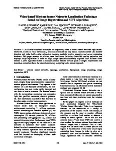
5.2.4. Time of Arrival (TOA). In TOA, speed of wavelength and time of radio signals travelling between anchor node and unlocalized node is measured to estimate the location of unlocalized node [13]. GPS uses TOA, and it is a highly accurate technique; however, it requires high processing capability. We generated some interesting results by comparing few localization techniques. The results are based on our observations and analysis. Figure 3 shows cost of four localization techniques, and it is observed that GPS- and TOA-based systems are more expensive as compared with DV hop and RSSI. Figure 4 represents accuracy comparison of different localization techniques. It is observed that localization mechanisms equipped with GPS systems are highly accurate. Such mechanisms are needed for WSNs, which are energy efficient. Figure 5 shows comparison of energy efficiency of different localization mechanisms. GPS-based localization mechanisms are less energy efficient while RSSI-based mechanisms are highly energy efficient.

6. Analysis and Discussion WSN has many constraints such as node size, energy, and cost. It is indeed necessary to consider these constraints before designing any localization mechanism. Nodes communication and data transmission take much power and consume more energy. Many localization algorithms have been proposed; however, most of them are application specific. Localization algorithm designed for one application is not

6


Accuracy

As mentioned above, TWR measures the round-trip time of signal transmission between two nodes. The emission of frames is triggered, and the process is controlled by MAC layer. The principle of TWR to calculate different time stamps between two nodes is presented in the following equation [44]: 𝐷𝐴,𝐵 = V ⋅


TOA DV hop

Energy

Figure 4: Accuracy comparison of different localization mechanisms.


TOA DV hop

Figure 5: Energy efficiency comparison of different localization mechanisms.

necessarily suitable for other applications of WSNs. Similarly, some localization techniques are for mobile sensor nodes which are not suitable for static sensors. When message travels from one node to another, the range is estimated by measuring time of flight of radio frequency. When time of flight of radio frequency is used with two messages, it is known as two-way ranging (TWR) technique [36]. In TWR mechanism, sensor network starts with at least three anchor nodes which are used as reference for unlocalized nodes [37–39]. Clock synchronization is not necessary because anchor and unlocalized nodes have their own reference clocks [40–42]. When unlocalized nodes become localized through trilateration method, they can localize other unlocalized nodes. The process continues until all unlocalized nodes become localized. To achieve high level of accuracy, nodes can refine their positions. Distance or range is estimated by measuring the round-trip time of signal transmission between anchor and unlocalized nodes [43]. TWR is suitable for WSNs because it is of low cost having less hardware requirements with less energy consumption.

(𝑡4 − 𝑡1 ) − (𝑡3 − 𝑡2 ) , 2

(6)

where V is the speed of light (radio signals), 𝑡4 and 𝑡2 are reception instants, and 𝑡1 and 𝑡3 are emission instants. Clock synchronization is not a problem in this technique because each node has its own local clock and time stamps are calculated on these local clocks. When distance is measured by this formula, relatively accurate location can be estimated. Several authors proposed different protocols to analyze convergence speed and evaluate the communication cost related to energy. Different mechanisms are used to address some important issues such as the convergence conditions to achieve network wide localization, beginning and termination of the location propagation process, advantage of the broadcast nature of radio communications, and cooperation of nodes to reduce the number of exchanged messages and so energy consumption. TWR has some issues such as clock drift in cheap sensor nodes, different response delays of nodes, and channel impairments. In this section, we discuss the following three important protocols. (i) Beacon Protocol. In beacon protocol, anchor node initiates the localization process. Localization wave originates from the center of the network and progresses towards the network boundaries. When this process stops, there is no way to provide localization facility to newly added nodes. (ii) Continuous Ranging Protocol. In continuous ranging protocol, unlocalized node starts localization process, and its drawback is that unlocalized node sends range message even if localization wave still does not arrive. (iii) Optimized Beacon Protocol. Optimized beacon protocol is the same as beacon protocol in which anchor nodes send range messages. However, when unlocalized node overhears three range messages, it starts localization process without waiting for neighbor node. When unlocalized node becomes localized node, it can localize other nodes as well. Analysis shows that beacon protocol achieves the shortest delay and optimized beacon protocol requires fewer messages as compared with beacon and continuous ranging protocols. If estimation of location of node results in an error which is estimated by three neighbors’ nodes, it decreases the accuracy of localization. The reason is that such error propagates for further localization process, so overall accuracy is compromised. Similarly, security of WSNs at various layers is a challenging task. Localization of sensor nodes has numerous issues, and research community is trying to resolve them. In WSNs,


7

Table 1: Comparison of different localization techniques. Technique GPS GPS free Centralized based Decentralized based RSSI TOA (using ultrasonic pulse) TDOA AOA DV hop APIT

Cost High Low Depends Depends Low High Low High Low Medium

Accuracy High Medium High Low Medium Medium High Low Medium Medium

localization is an interesting research area, and still it has a lot of room for new researchers. (i) During the designing of localization algorithm, designers must consider low cost of power, hardware, and deployment of localization algorithm. (ii) Localization of sensor nodes using GPS is not suitable, because it is less energy efficient and expensive; it needs large size of hardware and has a line of sight problem. If GPS is installed on every node, then it increases the node size and deployment cost. Furthermore, GPS is not energy efficient as it consumes a lot of energy and not suitable for a network like WSN. (iii) It is more challenging to design localization system for WSN as compared with other networks. As in WSNs, it is important to consider all of the limitations such as battery power, low processing, limited memory, low data rates, and small size. (iv) In localization schemes, the problem of line of sight (LOS) can cause handling errors. (v) Accuracy is highly important factor in all localization techniques. Localization accuracy is compromised when position of node is wrongly estimated. When a node localizes itself with wrong information of coordinates and propagates wrong information throughout the network, overall accuracy of the localization process is decreased. (vi) Node density is an important factor in designing localization algorithm. For example, in beacon nodebased algorithms, beacon node density should be high for accurate localization, whereas if node density is low, then accuracy is decreased and localization algorithms cannot perform well. (vii) In mobile WSNs, nodes may leave and move to another location. In such case, topological changes may occur. In mobile WSNs, scalable mechanism is needed which is capable to cater topological changes. Furthermore, it is very difficult to estimate again and again position of node which is mobile in nature. Mobile nodes are continuously in motion. (viii) Fewer Number of Beacon Nodes can be built means that localization accuracy is improved and accurate

Energy efficient Less Medium Less High High Less High Medium High High

Hardware size Large Small Depends Depends Small Large Less complex, may be large Large Small Medium

as number of beacon nodes increases, but localization algorithm should be accurate with fewer number of beacon nodes. (ix) 3D Space. Localization should be suitable for deployment in actual 3D space. (x) Universal Nature. Algorithm should be designed not only for one specific application but for others as well. If algorithm is designed for indoor environments, it should also work for outdoor environments. Table 1 presents comparison of different localization techniques.

7. Conclusions WSNs have many applications in which sensor nodes collect data from particular location and process it. However, it is an important task to know the location of data from where it is collected. Localization is a mechanism in which nodes are located. There are many approaches for localization; however, such approaches are desirable which are capable to take care of limited resources of sensor nodes. In this paper, we explained different localization techniques in detail. Rangefree, range-based, and TWR techniques are deeply analyzed.

Acknowledgments The authors extend their appreciation to the Research Centre, College of Applied Medical Sciences and to the Deanship of the Scientific Research at King Saud University for funding this paper.

References [1] I. F. Akyildiz, W. Su, Y. Sankarasubramaniam, and E. Cayirci, “Wireless sensor networks: a survey,” Computer Networks, vol. 38, no. 4, pp. 393–422, 2005. [2] J. Yick, B. Mukherjee, and D. Ghosal, “Wireless sensor network survey,” Computer Networks, vol. 52, no. 12, pp. 2292–2330, 2008. [3] S. Gowrishankar, T. G. Basavaraju, D. H. Manjaiah, and S. K. Sarkar, “Issues in wireless sensor networks,” in Proceeding of the World Congress on Engineering (WCE ’08), vol. 1, London, UK, July 2008.

8 [4] N. Correal and N. Patwari, Wireless sensor network: challenges and opportunities, Florida Communication Research Lab, Gainesville, Fla, USA, 2001. [5] D. Ganesan, A. Cerpa, W. Ye, Y. Yu, J. Zhao, and D. Estrin, “Networking issues in wireless sensor networks,” Journal of Parallel and Distributed Computing, vol. 64, no. 7, pp. 799–814, 2004. [6] B. Sundararaman, U. Buy, and A. D. Kshemkalyani, “Clock synchronization for wireless sensor networks: a survey,” Ad Hoc Networks, vol. 3, no. 3, pp. 281–323, 2005. [7] I. F. Akyildiz and I. H. Kasimoglu, “Wireless sensor and actor networks: research challenges,” Ad Hoc Networks, vol. 2, no. 4, pp. 351–367, 2004. [8] J. A. Stankovic, “Research challenges for wireless sensor networks,” ACM SIGBED Review, vol. 1, no. 2, pp. 9–12, 2004. [9] G. Mao, B. Fidan, and B. D. O. Anderson, “Wireless sensor network localization techniques,” Computer Networks, vol. 51, no. 10, pp. 2529–2553, 2007. [10] A. Savvides, C.-C. Han, and M. B. Strivastava, “Dynamic finegrained localization in ad-hoc networks of sensors,” in Proceedings of the 7th Annual International Conference on Mobile Computing and Networking (MobiCom ’01), pp. 166–179, Rome, Italy, July 2001. [11] A. Savvides, H. Park, and M. B. Srivastava, “The n-hop multilateration primitive for node localization problems,” Mobile Networks and Applications, vol. 8, no. 4, pp. 443–451, 2003. [12] F. Hu and X. Cao, Wireless Sensor Networks: Principles and Practice, Auerbach, Boca Raton, Fla, USA, 1st edition, 2010. [13] R. Manzoor, Energy efficient localization in wireless sensor networks using noisy measurements [M.S. thesis], 2010. [14] L. E. W. Van Hoesel, L. Dal Pont, and P. J. M. Havinga, Design of an Autonomous Decentralized MAC Protocol for Wireless Sensor Networks, Centre for Telematics and Information Technology, University of Twente, Enschede, The Netherlands. [15] M. A. Perillo and W. B. Heinzelman, “Wireless sensor network protocols,” 2004. [16] A. Youssef and M. Youssef, “A taxonomy of localization schemes for wireless sensor networks,” in Proceedings of the International Conference on Wireless Networks (ICWN ’07), pp. 444–450, Las Vegas, Nev, USA, 2007. [17] K. Langendoen and N. Reijers, “Distributed localization in wireless sensor networks: a quantitative comparison,” Computer Networks, vol. 43, no. 4, pp. 499–518, 2003. [18] D. Moore, J. Leonard, D. Rus, and S. Teller, “Robust distributed network localization with noisy range measurements,” in Proceedings of the 2nd International Conference on Embedded Networked Sensor Systems (SenSys ’04), pp. 50–61, November 2004. [19] C. Savarese, J. M. Rabaey, and K. Langendoen, “Robust positioning algorithms for distributed ad-hoc wireless sensor networks,” in Proceedings of the 2002 USENIX Annual Technical Conference on General Track, pp. 317–327, USENIX Association, Berkeley, Calif, USA, 2002. [20] J. Liu, Y. Zhang, and F. Zao, “Robusr distributed node localization with error management,” in Proceeding of the 7th ACM International Symposium on Mobile Ad-Hoc Networking and Computing (MobiHoc ’06), pp. 250–261, Florence, Italy, May 2006. [21] S. Qureshi, A. Asar, A. Rehman, and A. Baseer, “Swarm intelligence based detection of malicious beacon node for secure localization in wireless sensor networks,” Journal of Emerging


[22]

[23]

[24]

[25] [26]

[27]

[28]

[29]

[30]

[31]

[32]

[33]

[34]

[35]

[36]

Trends in Engineering and Applied Sciences, vol. 2, no. 4, pp. 664–672, 2011. N. Bulusu, J. Heidemann, and D. Estrin, “GPS-less low-cost outdoor localization for very small devices,” IEEE Personal Communications Magazine, vol. 7, no. 5, pp. 28–34, 2000. E. Kim and K. Kim, “Distance estimation with weighted least squares for mobile beacon-based localization in wireless sensor networks,” IEEE Signal Processing Letters, vol. 7, no. 6, pp. 559– 562, 2010. T. He, C. Huang, B. M. Blum, J. A. Stankovic, and T. Abdelzaher, “Range-free localization schemes for large scale sensor networks,” in Proceedings of the 9th ACM Annual International Conference on Mobile Computing and Networking (MobiCom ’03), pp. 81–95, September 2003. T. He, C. Huang, B. M. Blum, J. A. Stankvic, and T. Abdelzaher, “Range free localization,” 2006. Q. Huang and S. Selvakennedy, “A range-free localization algorithm for wireless sensor networks,” in Proceedings of the IEEE 63rd Vehicular Technology Conference (VTC ’06), pp. 349–353, School of InformationTechnologies, Melbourne, Australia, July 2006. R. Stoleru, T. He, and J. A. Stankovic, “Range free localization,” in Secure Localization and Time Synchronization for Wireless Sensor and Ad Hoc Networks, vol. 30, pp. 3–31, Springer, Berlin, Germany, 2007. L. Doherty, K. S. J. Pister, and L. El Ghaoui, “Convex position estimation in wireless sensor networks,” in Proceedings of the 20th Annual Joint Conference of the IEEE Computer and Communications Societies (INFOCOM ’01), pp. 1655–1663, April 2001. A. Savvides, C. Han, and M. Srivastava, “Dynamic fine-grained localization in ad-hoc networks of sensors,” in Proceedings of the 7th ACM Annual International Conference on Mobile Computing and Networking (MobiCom ’01), pp. 166–179, Rome, Italy, July 2001. A. Savvides, H. Park, and M. B. Srivastava, “The bits and flops of the n-hop multilateration primitive for node localization problems,” in Proceedings of the 1st ACM International Workshop on Wireless Sensor Networks and Applications (WSNA ’02), pp. 112–121, September 2002. A. Nasipuri and K. Li, “A directionality based location discovery scheme for wireless sensor networks,” in Proceedings of the 1st ACM International Workshop on Wireless Sensor Networks and Applications (WSNA ’02), pp. 105–111, September 2002. N. Patwari, A. O. Hero, M. Perkins, N. S. Correal, and R. J. O’Dea, “Relative location estimation in wireless sensor networks,” IEEE Transactions on Signal Processing, vol. 51, no. 8, pp. 2137–2148, 2003. D. Niculescu and B. Nath, “Ad hoc positioning system (APS) using AOA,” in Proceedings of the 22nd Annual Joint Conference on the IEEE Computer and Communications Societies (INFOCOM ’03), pp. 1734–1743, San Francisco, Calif, USA, April 2003. D. Liu, P. Ning, and W. Du, “Detecting malicious beacon nodes for secure location discovery in wireless sensor networks,” in Proceedings of the 25th IEEE International Conference on Distributed Computing Systems ((ICDCS ’05)), pp. 609–619, June 2005. J. Bachrach and C. Taylor, Localization in Sensor Networks, Massachusetts Institute of Technology, Cambridge, Mass, USA, 2004. S. Tanvir, Energy efficient localization for wireless sensor network [Ph.D. thesis], 2010.

International Journal of Distributed Sensor Networks [37] R. Hach, “Symmetric double sided two-way ranging,” IEEE 802. 15. 4a, Ranging Subcommittee, 2005. [38] L. J. Xing, L. Zhiwei, and F. C. P. Shin, “Symmetric double side two way rangingwith unequal reply time,” in Proceedings of the IEEE 66th Vehicular Technology Conference (VTC ’07), pp. 1980– 1983, Baltimore, Md, USA, October 2007. [39] J. Decuir, “Two way time transfer based ranging,” Contribution to the IEEE 802. 15. 4a, Ranging Subcommittee, 2004. [40] R. Manzoor, Energy efficient localization in wireless sensor networks using noisy measurements [M.S. thesis], 2010. [41] R. Hach, “Symmetric double sided two-way ranging,” IEEE 802. 15. 4a, Ranging Subcommittee, 2005. [42] N. Hajlaoui, I. Jabri, and M. B. Jemaa, “Experimental performance evaluation and frame aggregation enhancement in IEEE 802.11n WLANs,” International Journal of Communication Networks and Information Security, vol. 5, no. 1, pp. 48–58, 2013. [43] S. Tanvir, E. Schiller, B. Ponsard, and A. Duda, “Propagation protocols for network-wide localization based on two-way ranging,” in Proceedings of the IEEE Wireless Communications and Networking Conference (WCNC ’10), Sydney, Australia, April 2010. [44] S. Tanvir, F. Jabeen, M. I. Khan, and B. Ponsard, “On propagation properties of beacon based localization protocol for wireless sensor networks,” Middle-East Journal of Scientific Research, vol. 12, no. 2, pp. 131–140, 2012.

9