Localized Content-Based Image Retrieval Using Semi-Supervised Multiple Instance Learning? Dan Zhang1 , Zhenwei Shi2 , Yangqiu Song1 , Changshui Zhang1 1. State Key Laboratory on Intelligent Technology and Systems Tsinghua National Laboratory for Information Science and Technology (TNList), Department of Automation,Tsinghua University, Beijing 100084, China 2. Image Processing Center, School of Astronautics, Beijing University of Aeronautics and Astronautics, Beijing 100083, P.R. China
[email protected],
[email protected],
[email protected],
[email protected]
Abstract. In this paper, we propose a Semi-Supervised Multiple-Instance Learning (SSMIL) algorithm, and apply it to Localized Content-Based Image Retrieval(LCBIR), where the goal is to rank all the images in the database, according to the object that users want to retrieve. SSMIL treats LCBIR as a Semi-Supervised Problem and utilize the unlabeled pictures to help improve the retrieval performance. The comparison result of SSMIL with several state-of-art algorithms is promising.
1
Introduction
Much work has been done in applying Multiple Instance Learning (MIL) to Localized Content-Based Image Retrieval (LCBIR). One main reason is that, in LCBIR, what a user wants to retrieve is often an object in a picture, rather than the whole picture itself. Therefore, in order to tell the retrieval system what he really wants, the user often has to provide several pictures with the desired object on it, as well as several pictures without this object, either directly or through relevance feedback. Then, each picture with the desired object is treated as a positive bag, while the other query pictures will be considered as negative ones. Furthermore, after using image segmentation techniques to divide the images into small patches, each patch represents an instance. In this way, the problem of image retrieval can be converted to an MIL one. The notion of Multi-Instance Learning was first introduced by Dietterich et al. [1] to deal with the drug activity prediction. A collection of different shapes of the same molecule is called a bag, while its different shapes represent different instances. A bag is labeled positive if and only if at least one of its instances is positive; otherwise, this bag is negative. This basic idea was extended by several following works. Maron et al. [2] proposed another MIL algorithm - Diverse Density (DD). They tried to find a target in the feature space that resembled ?
The work was supported by the National Science Foundation of China (60475001, 60605002)
positive instance most, and this target was called a concept point. Then they applied this method to solve the task of natural scene classification [3]. Zhang and Goldman [6] combined Expectation Maximization with DD together and developed an algorithm EM-DD, which was much more efficent than the previous DD algorithm, to search for the desired concept. They extended their idea in [7] and made some modifications to ensemble the different concept points returned by EM-DD with different initial values. This is reasonable, since the desired object can not be described by only one concept point. Andrew et al. [10] used a SVM based method to solve the MI problem. Then, they developed an efficient algorithm based on linear programming boosting [11]. Y. Chen et al. [4] combined EM-DD and SVM, and devised DD-SVM. Recently, P.M. Cheung et al.[9] give a regularized framework to solve this problem. Z. H. Zhou etc. [15], also initiate some research on Multiple-Instance Multiple-Label problem and apply it to scene classification. All the above works assume that each negative bag should not contain any positive instance. But there may exist exceptions. After the image segmentation, the desired object may be divided into several different patches. The pictures without this object may also contain a few particular patches that are similar to that of the object and should not be retrieved. So, negative bags may also contain positive instances, if we consider each patch as an instance. Based on this assumption, Y. Chen et al. [5] recently devised a new algorithm called MultipleInstance Learning via Embedded Instance Selection (MILES) to solve multiple instance problems. So far, some developments of MIL have been reviewed. When it comes to LCBIR, one natural problem is that users are often unwilling to provide so many labeled pictures, and therefore the inadequate number of labeled pictures poses a great challenge to the existing MIL algorithms. Semi-Supervised algorithms are just devised to handle the situation when the labeled information is inadequate. Some typical semi-supervised algorithms include Semi-Supervised SVM [13], Transductive SVM [12], graph-based semi-supervised learning [14], etc. How to convert a standard MIL problem to a Semi-Supervised one has received some notices. Recently, R. Rahmani and S. Goldman combined a modified version of DD and graph-based semi-supervised algorithms together, and put forward the first graph-based Semi-Supervised MIL algorithm - MISSL[8]. They adopted an energy function to describe the likelihood of an instance being the concept points, and redefined the weights between different bags. In this paper, we propose a new algorithm - Semi-Supervised Multiple-Instance Learning (SSMIL) to solve the Semi-Supervised MIL problem, and the result is promising. Our paper is outlined as follows: in Section 2, the motivation of our algorithm will be introduced. In Section 3, we will give the proposed algorithm. In Section 4 the experimental results will be presented. In the end, a conclusion is given in Section 5.
2
Motivation
A bag can be mapped into a feature space determined by the instances in all the labeled bags. To be more precise, a bag B is embedded in this feature space as follows [5]: m(B) = [s(x1 , B), s(x2 , B), · · · , s(xn , B)]T (1) k Here, s(xk , B) = maxt exp(− ||btσ−2x || ). σ is a predefined scaling parameter. xk is the kth instance among all the n instances in the labeled bags and bt denotes the tth instance in the bag B. Then, the whole labeled set can be mapped to such a matrix:
+ − − [m+ 1 , · · · , ml + , m1 , · · · , ml − ] + + − = [m(B ), · · · , m(B− 1 ), · · · , m(Bl+ ), m(B1 l− )] + − s(x1 , B1 ) · · · s(x1 , Bl− ) − 2 s(x2 , B+ 1 ) · · · s(x , Bl− ) = .. .. .. . . .
(2)
− n s(xn , B+ 1 ) · · · s(x , Bl− )
+ − − B+ 1 , . . . , Bl+ denote the bags labeled positive, while B1 , . . . , Bl− refer to the k negatively labeled bags. Each column represents a bag. If x is near some positive bags and far from some negative ones, the corresponding dimension is useful for discrimination. In MILES[5], a 1-norm SVM is trained to select features and get their corresponding weights from this feature space as follows :
min λ
w,b,ξ,η
n X k=1
+
|wk | + C1
l X i=1
−
ξi + C2
l X
ηj
j=1
+ s.t. (wT m+ i + b) + ξi ≥ 1, i = 1, . . . , l , − − (wT m− j + b) + ηj ≥ 1, j = 1, . . . , l ,
ξi , ηj ≥ 0, i = 1, . . . , l+ , j = 1, . . . , l−
(3)
Here, C1 and C2 reflect the loss penalty imposed on the misclassification of positive and negative bags, respectively. λ is a regularizer parameter, which controls the trade-off between the complexity of the classifier and the hinge loss. It can be seen that this formulation does not restrict all the instances in negative bags to be negative. Since the 1-norm SVM is utilized, a sparse solution can be obtained, i.e. in this solution, only a few wk in Eq. (3) are nonzero. Hence, MILES finds the most important instances in the labeled bags and their corresponding weights. MILES gives an impressive result on several data sets and has shown its advantages over several other methods, such as DD-SVM [4], MI-SVM [10]and k-means SVM [16], both in accuracy and speed. However, the image retrieval task is itself a Semi-Supervised problem - with only a few labeled pictures searching in a tremendous database. The utilization of the unlabeled pictures may actually improve the retrieval performance.
3 3.1
Semi-Supervised Multiple Instance Learning (SSMIL) The Formulation of Semi-Supervised Multiple Instance Learning
In this section, we give the formulation for Semi-Supervised Multiple Instance Learning. Our aim is to maximize margins not only on the labeled but the unlabeled bags. A straightforward way is to map both the labeled and unlabeled bags into the feature space determined by all the labeled bags, using Eq. (2). Then, we try to solve such an optimization problem: minw,b,ξ,η,ζ λ
n P
+
|wk | + C1
l P
−
ξi + C2
l P
ηj + C3
i=1 j=1 k=1 s.t. (wT m+ + b) + ξ ≥ 1, i = 1, · · · , l+ i i T − −(w mi + b) + ηj ≥ 1, j = 1, · · · , l− yu∗ (wT mu + b) + ζu ≥ 1, u = 1, · · · , |U | ξi , ηj , ζu ≥ 0, i = 1, · · · , l+ , j = 1, · · · , l− ,
|U P| u=1
ζu (4)
u = 1, · · · , |U | The difference between Eq. (3) and Eq. (4) is the appended penalty term imposed on the unlabeled data. C3 is the penalty parameter that controls the effect of unlabeled data, and yu∗ is the label assigned to the uth unlabeled bag during the training phase. 3.2
The Up-Speed of Semi-Supervised Multiple Instance Learning (UP-SSMIL)
Directly solving the optimization problem (4) is too time-consuming, because, in Eq. (4), all the unlabeled pictures are required to be mapped into the feature space determined by all the instances in the labeled bags and most of the time will be spent on the feature mapping step(Eq. (2)). In this paper, we try to up-speed this process and propose UP-SSMIL. After each labeled bag is mapped into the feature space by Eq. (2), all the unlabeled bags can also be mapped into this feature space according to Eq. (1). As mentioned in Section 2, one norm SVM can find the most important features, i.e. predominant instances in training bags. Hence, the dimension for each bag can be greatly reduced, with the irrelevant features being discarded. So, we propose using MILES as the first step to select the most important instances and mapping each bag B in both the labeled and unlabeled set into the space determined by these instances as follows: m(B) = [s(z1 , B), s(z2 , B), · · · , s(zv , B)]T
(5)
Here, z k is the kth selected instance and v denotes the total number of the selected instances. This is a supervised step. Then, we intend to use the unlabeled bags to improve the performance by optimize the feature weights of the
1. Feature Mapping 1: Map each labeled bag (into the feature space determined by the instances in the labeled bags, using Eq.(2). 2. MILES Training: Use 1-norm SVM to train a classifier, utilizing only the training bags. Then, each feature in the feature space determined by the training instances is assigned a weight, i.e. wk in Eq. (3). The regularizer in this step is denoted as λ1 . 3. Feature Selecting: Select the features with nonzero weights. 4. Feature Mapping 2: Map all the unlabeled and labeled bags into the feature space determined by the features selected from the previous step, i.e. the selected instances, using Eq. (5). 5. TSVM Training: Taking into account both the re-mapped labeled and unlabeled bags, use TSVM to train a classifier. The regularizer in TSVM is denoted as λ2 . 6. Classifying: Use this classifier to rank the unlabeled bags. Table 1. UP-SSMIL Algorithm
selected features. A Transductive Support Vector Machine (TSVM) [12] algorithm is employed to learn these weights. The whole UP-SSMIL algorithm can be depicted in Table 1. In this algorithm, TSVM is a 2-norm Semi-Supervised SVM. The reason why 1-norm Semi-Supervised SVM is not employed is that, after the feature selection step, the selected features are most relevant to the final solution. However, 1norm Semi-Supervised SVM favors the sparsity of w. Therefore, it is not used here.
4
Experiments
(a) SpriteCan
(b) WD40Can
Fig. 1. Some sample images in SIVAL dataset.
We test our method on SIVAL , which is obtained at www.cs.wustl.edu/∼sg/multiinst-data/. Some sample images are shown in Fig. (1). In this database, each
image is pre-segmented into around 30 patches. Color, texture and neighborhood features have already been extracted for each patch, and form a set of 30-dimension feature vectors. In our experiments, these features are normalized to be exactly in the range from 0 to 1, and the scaling parameter σ is chosen to be 0.5. Treat each picture as a bag, and each patch in this picture as an instance in this bag. The source code of MILES is obtained from [17], and TSVM is obtained from [18]. During each trial, 8 positive pictures are randomly selected from one category, and other 8 negative pictures are randomly selected as background pictures from the other 24 categories. The retrieval speed of UP-SSMIL is pretty fast. In my computer, for each round, UP-SSMIL takes only 25 seconds while SSMIL takes around 30 minutes. For convenience, only the results of UP-SSMIL are reported here. We will demonstrate below that it achieves the best performance on SIVAL database. In UP-SSMIL’s Training step in Table 1 and MILES (see Eq. (3)), λ1 is set to 0.2, C1 and C2 are set to 0.5. In UP-SSMIL’s TSVM Training step in Table 1 (for a detailed description of the parameters, see the reference of SVMlin [18]), λ2 is set to 0.1 The positive class fraction of unlabeled data is set to 0.01. The other parameters in SVMlin are all set to their default values. In the image retrieval, the ROC curve is a good measure of the performance. So, the area under ROC curve - AUC value is used here to measure the performance. All the results reported here are averaged over 30 independent runs, with a 95% confidence interval being calculated. The final comparison result is shown in Table 2. From this table, it can be seen that, compared with MISSL, among all the 25 categories, UP-SSMIL performs better than MISSL for most categories, with only a few categories worse than MISSL. This may be due to two reasons. For one thing, MISSL uses inadequate number of pictures to learn the likelihood for each instance being positive and the “steepness factor” in MISSL is relatively hard to determine. These may lead to an inaccurate energy function. For another, on the graph level, MISSL uses just one vertex to represent all the negative training vertexes, and assumes the weights connecting from this vertex to all the unlabeled vertexes to be the same, which will result in some inaccuracy as well. Furthermore, after the pre-calculation of the distances between different instances, MISSL takes 30-100 seconds to get a retrieval result, while UP-SSMIL takes no more than 30 seconds without the need to calculate these distances. This is quite understandable, In the first Feature Mapping Step in Table 1, UP-SSMIL only need to calculate the distances within the training bags. Since the number of query images is so small, this calculation burden is relatively light. Then, after the features being selected, the unlabeled bags only need to be mapped into the space determined by these few selected features. In our experiments, this dimension can be reduced to around 10. So, the calculation cost of the second Feature Mapping step in Table 1 is very low. With the dimensions being greatly reduced, TSVM gets the solution relatively fast. Compared with other supervised methods, such as MILES, Accio [7] and Accio+EM [7]. The performance of UP-SSMIL is also quite promising. Some
comparisons result with its supervised opponent–MILES are provided in Fig. 2. We illustrate how the learning curve will change when both the number of labeled pictures(|L|) and the number of unlabeled pictures(|U |) vary. It can be seen that the performance of UP-SSMIL always outperforms its supervised opponent.
5
Conclusions
In this paper, we propose a semi-supervised SVM framework of Multiple Instance algorithm - SSMIL. It uses the unlabeled pictures to help improve the performance. Then, UP-SSMIL is presented to accelerate the retrieval speed. In the end, we demonstrate on SIVAL database its superior performances.
UP-SSMIL MISSL MILES Accio! Accio!+EM FabricSoftenerBox 97.2±0.7 97.7±0.3 96.8±0.9 86.6±2.9 44.4±1.1 CheckeredScarf 95.5±0.5 88.9±0.7 95.1±0.8 90.8±1.5 58.1±4.4 FeltFlowerRug 94.6±0.8 90.5±1.1 94.1±0.8 86.9±1.6 51.1±24.8 WD40Can 90.5±1.3 93.9±0.9 86.9±3.0 82.0±2.4 50.3±3.0 CockCan 93.4±0.8 93.3±0.9 91.8±1.3 81.5±3.4 48.5±24.6 GreenTeaBox 90.9±1.9 80.4±3.5 89.4±3.1 87.3±2.9 46.8±3.5 AjaxOrange 90.1±1.7 90.0±2.1 88.4±2.8 77.0±3.4 43.6±2.4 DirtyRunningShoe 87.2±1.3 78.2±1.6 85.6±2.1 83.7±1.9 75.4±19.8 CandleWithHolder 85.4±1.7 84.5±0.8 83.4±2.3 68.8±2.3 57.9±3.0 SpriteCan 84.8±1.1 81.2±1.5 82.1±2.8 71.9±2.4 59.2±22.1 JulisPot 82.1±2.9 68.0±5.2 78.8±3.5 79.2±2.6 51.2±24.5 GoldMedal 80.9±3.0 83.4±2.7 76.1±3.9 77.7±2.6 42.1±3.6 DirtyWorkGlove 81.9±1.7 73.8±3.4 80.4±2.2 65.3±1.5 57.8±2.9 CardBoardBox 81.1±2.3 69.6±2.5 78.4±3.0 67.9±2.2 57.8±2.9 SmileyFaceDoll 80.7±1.8 80.7±2.0 77.7±2.8 77.4±3.2 48.0±25.8 BlueScrunge 76.7±2.6 76.8±5.2 73.2±2.8 69.5±3.3 36.3±2.5 DataMiningBook 76.6±1.9 77.3±4.3 74.0±2.3 74.7±3.3 37.7±4.9 TranslucentBowl 76.3±2.0 63.2±5.2 74.0±3.1 77.5±2.3 47.4±25.9 StripedNoteBook 75.1±2.6 70.2±2.9 73.2±2.5 70.2±3.1 43.5±3.1 Banana 69.2±3.0 62.4±4.3 66.4±3.4 65.9±3.2 43.6±3.8 GlazedWoodPot 68.6±2.8 51.5±3.3 69.0±3.0 72.7±2.2 51.0±2.8 Apple 67.8±2.7 51.1±4.4 64.7±2.8 63.4±3.3 43.4±2.7 RapBook 64.9±2.8 61.3±2.8 64.6±2.3 62.8±1.7 57.6±4.8 WoodRollingPin 64.1±2.1 51.6±2.6 63.5±2.0 66.7±1.7 52.5±23.9 LargeSpoon 58.6±1.9 50.2±2.1 57.7±2.1 57.6±2.3 51.2±2.5 Average 80.6 74.8 78.6 74.6 50.3 Table 2. Average AUC values with 95% confidence intervals, with 8 randomly selected positive and 8 randomly selected negative pictures
SpriteCan |U|=1500−|L|
SpriteCan |L|=16
0.92 0.86
0.9
0.84
0.88 AUC value
AUC value
0.82
0.86 0.84
0.8 0.78
MILES
0.76
UP−SSMIL
0.74
0.82
MILES
0.8 0.78
UP−SSMIL
0.72
20
30 40 50 60 Number of labeled pictures (|L|)
70
0.7
80
200
400 600 800 Number of unlabeled pictures (|U|)
(a)
(b)
WD40can |U|=1500−|L|
WD40Can |L|=16
0.96
0.92
0.95
0.91 0.9
0.94
0.89 AUC value
AUC value
0.93 0.92 0.91 0.9
0.88 0.87 0.86 0.85
0.89 0.88 0.87
1000
20
MILES
0.84
UP−SSMIL
0.83
30 40 50 60 Number of labeled pictures (|L|)
(c)
70
80
0.82
MILES UP−SSMIL 200
400 600 800 Number of unlabeled pictures (|U|)
1000
(d)
Fig. 2. The comparison result between UP-SSMIL and MILES
References 1. T. G. Dietterich, R. H. Lathrop, and T. Lozano-P¨ erez: “Solving the Multiple Instance Problem with Axis-Parallel Rectangles,” in Artificial Inteligence, vol. 1446, pp.1-8, (1998) 2. O. Maron and T. Lozano-P:¨ erez, “A Framework for Multiple-Instance Learning,” Advances in Neural Information Processing System 10, pp. 570-576, (1998) 3. O. Maron and A. L. Ratan: “Multiple-Instance Learning for Natural Scene Classification,” in Proc. 15th Int’l Conf. Machine Learning, pp. 341-349, (1998) 4. Y. Chen and J. Z. Wang: “Image Categorization by Learning and Reasoning with Regions,” J. Machine Learning Research, vol. 5, pp. 913-939, (2004) 5. Y. Chen, Jinbo Bi, and James Z. Wang: “MILES: Multiple-Instance Learning via Embedded Instance Selection,” in IEEE Transatctions on Pattern Analysis and Machine Intelligence, vol. 28, No.12, (2006) 6. Q. Zhang and S. Goldman: “EM-DD: An improved Multiple-Instance Learning,” in Advances in Neural Information Processing System 14, pp.1073-1080, (2002) 7. R. Rahmani, S. Goldman, H. Zhang, et al: “Localized Content-Based Image Retrieval,” in Proceedings of ACM Workshop on Multimedia Image Retrieval , (2005) 8. R. Rahmani, S. Goldman: “MISSL: Multiple-Instance Semi-Supervised Learning,” in Proc. 23th Int’l Conf. Machine Learning, pp. 705-712, (2006) 9. Pak-Ming Cheung, James T.Kwok: A Regularization Framework for MultipleInstance Learning, ICML(2006)
10. S. Andrews, I. Tsochantaridis and T. Hofmann: “Support Vector Machines for Multiple-Instance Learning,” in Advances in Neural Information Processing System 15, pp. 561-568, (2003) 11. S. Andrews, T. Hofmann: “Multiple Instance Learning via Disjunctive Programming Boosting,” in Advances in Neural Information Processing System 16, pp. 65-72, (2004) 12. T. Joachims: “Transductive Inference for Text Classification using Support Vector Machine,” in Proc. 16th Int’l Conf. Machine Learning, pp.200-209, (1999) 13. Bennett K. P., Demiriz A.: “Semi-supervised sup- port vector machines.,” in Advances in Neural Information Processing System 11, pp.368-374, (1999) 14. Zhu, X.: “Semi-supervised learning literature survey,” in Technical Report 1530, Department of Computer Sci- ences, University of Wisconsin at Madison., (2006) 15. Z.H.Zhou, M.L. Zhang: “Multi-Instance Multi-Label Learning with Application to Scene Classification,” in Advances in Neural Information Processing System, (2006) 16. G. Csurka, C. Bray, C. Dance, and L. Fan: “Visual Categorization with Bags of Keypoints,” in Proc. ECCV ’04 Workshop Statistical Learning in Computer Vision, pp.59-74, (2004) 17. http://john.cs.olemiss.edu/∼ychen/MILES.html 18. http://people.cs.uchicago.edu/∼vikass/svmlin.html