vk E N(O, Qk); COV(Vt, 213) = Qk&-j. (21). e k E N(0, &); COV(ei, e3) .... [l] Harold L. Alexander. State estimation for dis- ... Nice, France, 1992. [B] Arthur Gelb.
Location Estimation using Delayed Measurements M. Bak, T. D. Larsen, M. N@rgaard*,N. A. Andersen, N. K. Poulsen*& 0. Ravn Department of Automation, Technical University of Denmark Building 326, DK-2800 Lyngby, Denmark
Abstract
a measurement will not reflect the current states of the system it observes and some caution should therefore be taken. For motion control and navigation it is vital continuously t o attain knowledge of location in order t o keep a vehicle near its desired path. In AGV applications odometry combined with vision is a widely used approach t o location estimation and has proven satisfactory performance [5], [8],[10]. However, the measurement delay handling is often neglected by using either sophisticated hardware, minimal image processing, predefined travelling paths or a stop & go strategy, where the AGV stops t o process measurements. The latter method has been applied in [2] for docking and navigation through a door. In some cases, though, this is not a feasible strategy and explicit handling of the time delay is necessary. The purpose of this paper is t o focus on the problem of dealing with significant time delays in state estimation using a Kalman filter. This is based on a fast and effective technique described in [7] where delayed measurements easily are incorporated in the state. The method is applied t o an AGV using odometry and vision for location estimation where sensor related time delays of 30-40 samples exist in the vision system. The sampling period is 40 ms. The paper is organized as follows: Section 2 gives a survey of existing techniques for handling the time delays and presents our technique, Section 3 describes the algorithms for for estimating the position and orientation of the AGV, section 4 shows the concept through experiments and finally, Section 5 summarizes the results and concludes.
When combining data from various sensors it is vital to acknowledge possible measurement delays. Furthermore, the sensor fusion algorithm, often a Kalman filter, should be modified in order to handle the delay. This paper examines different possibilities for handling delays and applies a new technique to a sensor fusion system for estamating the location of an Autonomous Guided Vehicle. The system fuses encoder and vision measurements in an extended Kalman filter. Results from experiments in a real environment are reported.
1
Introduction
In a complex control system more than one sensor is often needed to generate and maintain a reliable state estimate. Furthermore, the complexity of the computations in sensors will often introduce significant time delays from the acquisition to the availability of a measurement. This can be due t o signal and image processing, data transportation, laboratory tests, etc. Two examples of systems with delayed measurements are an Autonomous Guided Vehicle (AGV) using vision and a wastewater treatment plant using water samples. Vision is a versatile sensor often used in a location system for detecting natural or artificial guide marks but the recording of an image and the following image processing, that may require extensive computations, will introduce time delays. Faster and more advanced image equipment may decrease the delay but then again more intelligent and complex image algorithms will increase it. In a wastewater treatment plant the water quality is often monitored by doing comprehensive laboratory tests on water samples resulting in up t o several days delayed measurements. How to incorporate possible unknown time-varying delayed measurements in a state estimation can be non-trivial. As a consequence of sensor-related delays,
2
The presentation herein is based on the Kalman filter equations for a discrete linearized time-varying system with state vector x k , input vector uk and output vector yk. The following lists the equations for notational purpose [6].
*Department of Mathematical Modelling
0-7803-4484-7/98/$10.00 0 1998 IEEE
Delayed Measurements
180
A M C '98 - COIMBFU
Authorized licensed use limited to: Danmarks Tekniske Informationscenter. Downloaded on June 01,2010 at 11:00:43 UTC from IEEE Xplore. Restrictions apply.
System:
be carried out in one sample. Further, given a system where a d-sample delayed measurement arrives a t each sampling instance the filtering of a given time interval will be repeated d-times. This puts great demands on the processing unit. [l]proposes a method for how t o minimize the required computations in recalculating the filter by updating the covariance matrix P k and the state ?k a t different times. Given the covariance of the measurement, R k and the measurement matrix, CT are known at the time of acquisition, le - d, the covariance of the state, 9 ,can be updated a t sampling k - d and a t sampling k , a correction to the state can quite easily be made calculated and applied. The disadvantage of this method is that in the time interval k - d t o k the accuracy of the state is wrong (the P matrix has wrongly been updated) and this can lead t o misvalidation of other measurements arriving in the time interval. In [7] an extension to this method is proposed that avoids the problem of wrongly updating the covariance matrix by having two filters running in parallel. One filter runs with and one filter runs optimal without the updated covariance matrix P K .
In case a sensor has a time delay from the acquisition to the availability of a given measurement, the sensor’s output equation becomes:
where d is the number of delayed samples which is here assumed to be an integer. This means that the measurement is acquired at sampling k - d but are not available until sampling k .
2.1
2.2
Survey of Methods
Interpolating Measurements
As mentioned in section 2.1 the method for handling sensor-related delays by [ l ] requires the knowledge of the measurement matrix, Cf-d and the covariance matrix R k - d at the time of the acquisition. This might not be the case as with our AGV used for the experiments where the covariance on the vision measurements very much depend on the distance and the angle to the observed object, i.e. the uncertainty on the distance to an object is proportional with the actual distance. In order to avoid the computational expensive recalculation of the filter, a new method is needed. The following method is described in detail in [7] and shall here be adopted for our application. Basically, the idea is to interpolate the measurement so that it reflects current states rather than prior. Heuristically, this is done by modifying the measurement based on the change in the system state in the time interval from acquisition t o availability. This leads to the following interpolated measurement y i :
A number of methods are available for handling the sensor-related time delays such that the measurement reflects current system stsatesrather than prior. A well-known classical approach, mentioned in e.g. [6], is t o augment the state vector in such a way that c T - d d 2 k - d becomes a state. This way, the measurement does reflect a current state and the measurement update can be carried out as usual. The method is only convenient for constant and small time delays as the state vector is expanded by m x d states, where m is the dimension of the measurement. For time varying and large delays the method is time consuming due to the enlarged state vector and the implementation of the filter is made more difficult provided matrix symmetrical aspects are to be considered in order to reduce the computational burden. Another computational consuming method is recalculation of the filter upon arrival of a delayed measurement. Providing all measurements, state estimates, and covariance matrices have been stored since the acquisition of the measurement, the filter can be restarted a t sampling k - d and recalculated up to sampling k . This will obviously stress the filter for large delays since the recalculation preferably should
As a consequence of the adjustment, the Kalman Gain in the measurement update should be decreased to signal less belief in the incorporated measurement. [7] lists the following equation for the gain in case only
181
Authorized licensed use limited to: Danmarks Tekniske Informationscenter. Downloaded on June 01,2010 at 11:00:43 UTC from IEEE Xplore. Restrictions apply.
delayed measurements are fused:
Obviously, this is a simple computational cheap met hod. Figure 1: Guide mark used by vision.
3
Location Estimation for an AGV
and assuming that any noise vk attacking the system enters through uk, the equations (13)-( 15) can be rewritten as:
The following describes the location system onboard the AGV.
3.1
Odometry where f is nonlinear and given by (13)-(15). The noise vk comes from a number of sources such as uneven floors, wheel slippage, finite encoder resolution, misdetermined geometrical quantities (wheel radius, wheel distance), etc. This is further described in details in [4].
The two driving wheels are equipped with encoders and a t each sampling instance the encoder pulses provides information about the rotation of the wheel and thereby of the distance r, and rl driven by the right and the left wheel respectively. The reference point on the AGV is given by the mid point of the two wheels’ axis and this point’s displacement A S and rotational change A@ can be determined by:
as
=
3.2
rr + 5 2
Vision
The vision system on-board the AGV uses a 2dimensional guide mark of the type shown in Fig. 1 for location estimation. The dimension of the mark is 0.24 x 0.1 m . An image of a guide mark provides a measurement of the full state xk but due t o image recording and especially processing it will be delayed of 70-75 samples. This time delay is time-varying depending on the size and position of the guide mark and the number of potential guide marks in the image. Furthermore, it will be contaminated by some noise e k mainly due t o the discretation into pixels in the camera. This can be described by the following equation
where B is the distance between the two wheels. The position and orientation of the AGV in a twodimensional space can a t sampling instance k be reprewhere Xk, Yk sented by the triplet [ x k Yk 01, is the position and @k is the orientation or heading of the robot. The AGV’s position and rotation at sampling instance le 1 can be determined by the wellknown odometry model (see [ll]),providing the displacement and rotational change:
I’
+
where d is the number of delayed samples.
3.3
Fusion of Data with EKF
Equations (17) and (18) describe our location system and an extended Kalman filter (EKF) can now be applied for estimating the position and orientation by fusing the information from the encoders and t.he camera. Given encoder measurements, the state estimate gk can be updated using (17):
This model assumes the speed of the robot is constant between two sampling instances. By introducing a state vector x k and an input vector U k given as:
182
Authorized licensed use limited to: Danmarks Tekniske Informationscenter. Downloaded on June 01,2010 at 11:00:43 UTC from IEEE Xplore. Restrictions apply.
and the covariance of the state linearization of (17) : Pk+llk
=
FkPklkFT
Pk
4.1
is updated using a
-tG k Q k G ; ,
The AGV drive system consists of two DC motors mounted on the front wheels. They are equipped with encoders with an resolution of 800 pulses/turn. A standard commercial 512 x 512 pixel grey level type CCD camera is mounted on top of the AGV with an on-board CPU for image processing. The control and coordination of the AGV is handled by an on-board MVME-162A main board with a MC 68040 CPU running the OS-9 operating system. In order to evaluate the performance of the location system it is crucial to know the exact position and orientation of the AGV during an experiment. Here this is attained through a surveillance camera placed in the ceiling of the laoratory. The AGV is equipped with two light diodes, one on each side of the AGV, which are tracked with the surveillance camera. The position and orientation of the AGV can then be monitored with suitable image processing and knowledge of the camera’s internal parameters (such as focal length, center pixels, etc.) and the translation and rotation of the camera relative to some global reference coordinate system. This can be achieved using calibration tiles with known geometry. The recording of an image is synchronized with the AGV which allows for conformity in the ground truth and local AGV data. The uncertainty on the ground truth is estimated to be under 10 mm in position and 0.15’ in orientation. Due t o a limited field of view, this tracking system allows for tracking the AGV over an area of 1.75 m x 1.75 m . Additional cameras can easily be applied t o enlarge the tracking region but makes the calibration task somewhat more difficult. The following scenario is used for evaluation. The AGV travels parallel t o a wall on which a guide mark is placed. The camera is panned in order t o view the guide mark but otherwise kept in a constant position. The speed of the AGV is held under 0.15 m/s. Fig 2 shows the AGV trajectory. Before commencing the ex-
(20)
where F k and G k are Jacobian matrices of f k with respect to x k and uk respectively. Qk is the covariance of the process noise V k . The noise sequences { V k } and { e k } are assumed t o be white and Gaussian with the following properties: vk ek
E N(O, Q k ) ; COV(Vt, 213) = Q k & - j E N ( 0 , &); C O V ( e i , e 3 ) = &si-?,
Experimental Setup
(21) (22)
where dk is Kronecker’s delta function. Furthermore, v k and e k are assumed mutually independent, so that Cov(v,, ej) = 0 for all i, j . A delayed measurement is interpolated as described in section 2.2 and updated as in a standard Kalman filter (equations (3)-(5)) with measurement matrix c k = I. As the covariance of a vision measurement is modelled as a diagonal matrix, this implies that the components of the measurement X , Y and 0 are independent and accordingly can be split up in three measurements which can be processed one by one. This is advantageous regarding computational aspects and simplifies the implementation of a numerical stable algorithm which often builds on scalar measurements ~31. The vision system is limited in detection of guide marks due to a limited field of view for the camera and a constrained number of guide marks which implies interrupts in the measurements. Thus, the following algorithm has been applied.
No vision measurements. Only the time update is executed: $ k + l l k + l = ? k + l l k . One vision measurement. Interpolate the measurement and its covariance and execute both the time update and the measurement update. Additional vision measurements. As more than one guide mark may be in the field of view more than one vision measurement may arrive a t the same time. Here, the measurement update is executed once for each measurement.
Wall
F-Guide Mark
_____________---_----------
Figure 2: The AGV trajectory.
4
Experiments
periments, the systematical odometric errors has successfully been minimized by calibrating the distance between the wheels and the wheel diameters. This was
Experiments were carried out in the laboratory in order to examine and verify the location system. The test bed AGV is described in more details in [9].
183
Authorized licensed use limited to: Danmarks Tekniske Informationscenter. Downloaded on June 01,2010 at 11:00:43 UTC from IEEE Xplore. Restrictions apply.
carried out using the method in [4] and has resulted in a mean value positional drift of 2.8mm/m and orientational drift of 0.003'/m attained on an even floor without door steps or the like, which must be considered an unnatural working environment. The realistic drift is therefore higher. The parameters in the extended Kalman filter have been selected through calculations and experiments/observations. The stochastic errors effecting the odometry has been modelled in the covariance matrix Q and is selected as follows:
Finally, the initial values of the kalman filter (the state and the state error covariance matrix) have been selected as follows, assembling a realistic starting point: 2
- ?init
=
[
0.01m
(24)
Pinit = (0.01)2 x I.
(25)
Results
4.2
Fig. 5 and 6 show the location results from the first run where the delay is handled with the interpolation
method. Fig. 7 and 8 show the results where the delayed measurements are incorporated as they are. The effect from the time delay handling is only significant in the y state, which is the moving direction of the AGV. In case the heading of the AGV is changed during the time delay period, the effect is expected t o be much more crucial.
The covariance matrix, R k , for the vision measurements has been found by linearizing the set of equations used to transform the pixel-coordinates provided by the vision system into the AGV's position and orientation. Two temporary variables are used t o determine the uncertainty: the distance d,, from a guide mark to the AGV and the angle 0,, between the normal to a guide mark and the line-of-sight of the AGV camera. The uncertainty on the distance d,, is found to depend solely on the actual distance as shown in Fig. 3 while the uncertainty on the angle O,, is found to depend on both the distance and the actual angle as shown in Fig. 4. Knowing the uncertainty
0 02
'p
l l
E
I
-
I
p
Estimate Encoder Encoder
05
>
Y)
0
0
2
4
e
I 8
10
12
I4
time [secs]
Figure 3: Standard deviation for d,,
Figure 5: X and Y estimates with time delay handling.
.
5
"_?I
"
dm
In this paper different ways of approaching delayed measurements in a Kalman filter have been described. An algorithm for interpolating a delayed measurement minimizes the computational burden even for significant time delays. On our AGV, we have successfully applied this algorithm for dealing with delayed vision measurements in a locating system. By using an extended Kalman filter for fusing d a t a from encoders and camera, the location estimate shows satisfactory accuracy.
1-4
Figure 4: Standard deviation for O,,
Conclusions
.
on these two quantities, the covariance matrix Rk can be estimated.
184
Authorized licensed use limited to: Danmarks Tekniske Informationscenter. Downloaded on June 01,2010 at 11:00:43 UTC from IEEE Xplore. Restrictions apply.
:p --.
Estimate Vision Encoder
*,I
7
i
,
,
,
,
6
8
10
12
'Fl;
-3
Encoder
5 0
2
4
I
14
time [secs]
*
,
----
x -0 06
2
4
6
8
1
0
--1
2
1
4
2
4
6
8
1
0
1
2
1
, 1
*,
, 0
1
2
1
4
4
time [secs]
[8] Satoshi Murata and Takeshi Hirose. Onboard locating system using real-time image processing for a self-navigating vehicle. IEEE Transactions on Industrial Electronics, 40( 1), February 1993.
Figure 7: X and Y estimates without time delay handling.
Refer ences
[9] Ole Ravn and Nils A. Andersen. A test bed for experiments with intelligent vehicles. In Proceedings of the First Workshop on Intelligent Autonomous Vehicles, Southampton, England , 1995.
[l] Harold L. Alexander. State estimation for distributed systems with sensing delay. SPIE, 1470, 1991.
[a]
, 8
[7] Thomas D. Larsen, Niels K. Poulsen, Nils A. Andersen, and Ole Ravn. Incorporation of time delayed measurements in a discrete-time kalman filter. To appear, 1998.
* 0
6
[B] Arthur Gelb. Applied Optimal Estimation. The MIT Press, 1974.
time [secs]
0
4
[5] F. Chenavier and J. L. Crowley. Position estimation for a mobile robot using vision and odometry. In Proceedings of the 1992 IEEE International Conference on Robotics And Automation, Nice, France, 1992.
I
m
5-004
0
2
Figure 8: 0 estimate without time delay handling.
L
-0 08
0
time [secs]
Figure 6: 0 estimate with time delay handling. 0 02
---
[lo] E. Stella, G. Cirirelli, F. P. Lovergine, and A. Distante. Position estimation for a mobile robot using data fusion. In Proceedings of the 2995 IEEE International Symposium on Intelligent Control, Monterey, CA, USA, 1995.
Nils Andersen, Lars Henriksen, and Ole Ravn. Design of navigation and control for an agv. In Proceedings of the 2. IFAC Conference on Intelligent Autonomous Vehicles, Helsinki, 1995.
[11] C. Ming Wang. Location estimation and uncertainty analysis for mobile robots. In Proceedings of the 1988 International Conference on Robotics and Automation, Philadelphia, 1988.
[3] G.J. Bierman. Factorization Methods for Discrete Sequential Estimation. Academic Press, 1977.
[4] J. Borenstein and L. Feng. Measurement and correction of systematic odometry errors in mobile robots. IEEE Transactions on Robotics and Automation, 12(6), December 1996.
185
Authorized licensed use limited to: Danmarks Tekniske Informationscenter. Downloaded on June 01,2010 at 11:00:43 UTC from IEEE Xplore. Restrictions apply.