Logic-Based Methods for Optimization: A Tutorial - Semantic Scholar

Logic-Based Methods for Optimization: A Tutorial  J. N. Hooker

Graduate School of Industrial Administration Carnegie Mellon University, Pittsburgh, PA 15213 USA

December 1993

Abstract

Logic-based methods for optimization are increasingly attractive, for three main reasons. Logical inference algorithms have improved dramatically, connections between logic and mathematicalprogrammingare coming to light, and most importantly, logic-based methods solve models that combine logical and mathematical elements. This tutorial explains how integer programming problems can be naturally viewed as logical inference problems. It brie y describes a logic-based parallel of cutting plane theory and illustrates the solution of an IP by logic-based branch-and-bound. In particular it discusses and illustrates the generation of deep logic cuts. The tutorial also treats mixed integer programming from a logical point of view. It shows how integer variables may be eliminated entirely from the LP relaxation, and how logic cuts may be used to accelerate the solution. In particular it de nes a class of logic cuts that may cut o feasible solutions but do not aect the optimal solution. It illustrates the idea with an engineering application.

 Prepared for ORSA Computer Science Technical Section Conference, Williamsburg, VA, USA, January 1994. Supported in part by Oce of Naval Research Grant N00014-92-J-1028 and the Engineering Design Research Center at Carnegie Mellon University, funded by NSF grant 1-55093.

1

Contents

1 Introduction 2 Inequalities as Logical Propositions 3 Integer Programming as Logical Inference 4 An Integer Programming Example 5 A Branch-and-Cut Algorithm 6 Logic Processing 7 Branching Rules 8 Separation Algorithms 9 Solving the Relaxation 10 Example of Logic Cuts 11 Strong Cuts 12 Generation of Prime Cuts 13 Matching Problems 14 The Logic of Mixed Integer Programming 15 An MIP Example 16 An Example of Logic Cuts for MIP 17 Nonvalid Logic Cuts 18 A Processing Network Design Application

2

3 4 6 7 10 12 15 16 18 19 23 26 29 32 33 38 39 44

1 Introduction There is nothing new about logic-based techniques for optimization. Hammer and Rudeanu wrote a classic 1968 treatise [23] on boolean methods in operations research. Granot and Hammer [22] showed in 1971 how boolean methods might be used to solve integer programming problems. Although boolean methods have seen applications (logical reduction techniques, solution of certain combinatorial problems), they have not been accepted as a general-purpose approach to optimization. There seem to be two main reasons for this.

 They have not been demonstrated to be more eective than branch-and-cut. So there

has been no apparent advantage in converting a problem to boolean form.  The conversion to a boolean problem is itself hard.

The latter fact has been especially discouraging. The most straightforward way to convert an inequality constraint to boolean form, for instance, is to write it as an equivalent set of logical propositions. But the number of propositions can grow exponentially with the number of variables in the inequality. Consider for instance the following constraint from a problem in Nemhauser and Wolsey ([44], p. 465). 300x3 + 300x4 + 285x5 + 285x6 + 265x8 + 265x9 + 230x12 +230x13 + 190x14 + 200x22 + 400x23 + 200x24 + 400x25 +200x26 + 400x27 + 200x28 + 400x29 + 200x30 + 400x31  2700:

(1)

Barth [3] reports that this constraint expands to 117,520 nonredundant logical propositions, using the method of Granot and Hammer [22]. So for several years prospects for logic-based methods, as a general approach to optimization, looked bleak. But several factors have recently converged to make them much more attractive.

 Satis ability algorithms, potentially an important component of boolean methods, have

improved dramatically.  Recent work shows that is not necessary to expand an inequality constraint to the full list of logical propositions. This is analogous to generating all possible valid cutting planes for an integer programming problem. One generates only only separating cuts, and a similar option is available in logic-based algorithms.  There is a growing trend toward the merger of quantitative and logical elements into a single model, and logic-based methods are a natural approach to solving such models. The last factor is particularly important. Purely mathematical models (integer programming, etc.) are often unsuitable for messy problems without much mathematical structure, whereas pure logic models (PROLOG programs, etc.) do not capture the mathematical structure that does exist and are consequently hard to solve. Historically, solution techniques for 3

the two types of models have been unrelated. A technique that solves both opens the door to a wider variety of tractable models. Logic-based optimization also serves a heuristic function of providing a whole new perspective on optimization problems. In fact, it is in some ways more natural to view a pure IP problem as a logical inference problem rather than a polyhedral problem. Similarly, the integer variables of an MILP problem can be viewed as arti cial devices that can just as well be eliminated. Even if the particular algorithms described here are not suitable for a given problem, the logical point of view they represent may suggest algorithms that are. Logic-based methods provide not only another point of view but an entire body of theory and algorithms that parallels the classical material. Linear relaxations, cutting planes, facetde ning cuts, convex hulls, etc., all have logical parallels.

2 Inequalities as Logical Propositions The rst step toward a logic-based treatment of optimization is to regard inequality constraints as logical propositions.1 The 0-1 inequality 3x1 ? 2x2 + x3  2

(2)

is satis ed by exactly the same binary vectors (x1; x2; x3) as the logical proposition,

x1 ^ (x2 _ x3):

(3)

In (3) the variables xj are atomic propositions that are either true (denoted by xj = 1) or false (xj = 0). The symbol ^ means `and,' _ means `or,' and xj means `not-xj .' (2) makes the same statement as (3) because the left-hand side of (2) is greater than or equal to 2 exactly when (3) is true: x1 x2 x3 3x1 ? 2x2 + x3 x1 ^ (x2 _ x3) 0 0 0 0 0 1 0 0 0 1 ?2 0 0 1 0 0 1 1 ?1 0 3 1 1 0 0 4 1 1 0 1 1 1 0 1 0 2 1 1 1 1 The proposition (3) can be regarded as a boolean function of (x1; x2; x3) because it delivers a boolean value (1 or 0 for true or false) for every value of (x1; x2; x3). Not every boolean function is equivalent to a linear inequality in this way. For instance, the proposition (x1 ^ x2 ) _ (x1 ^ x2) (which can be written x1  x2) is equivalent to no 0-1 linear inequality in the variables x1 ; x2. A boolean function that is equivalent to some linear inequality is a threshold function. Threshold functions are surprisingly hard to characterize and have been studied intensively, primarily by electrical engineers [50]. The characterization issue is not relevant here, however. 1 I will assume throughout that inequalities have integral coecients.

4

Since inequalities are logical propositions, the usual relations among propositions apply to inequalities. An inequality I1 implies another I2 if all the 0-1 vectors satisfying I1 also satisfy I2 . Two inequalities are equivalent if they imply each other. Various sorts of domination between inequalities have been de ned and should be distinguished from implication. For instance, one might say that ax   dominates bx  when all real vectors x satisfying the former satisfy the latter. This is equivalent to saying that b = a and   for some  > 0. Thus 3x1 ? 2x2 + x3  2 implies x1  1 but does not dominate it, since (x1; x2; x3) = (1=2; 0; 1=2) satis es the former but not the latter. Also, equivalent inequalities need not be positive multiplies of one another, as in the case of x1  1 and 2x1  1. A system of 0-1 inequalities Ax  a implies an inequality bx  when all 0-1 solutions of the former satisfy the latter. But this is precisely what is meant by saying that bx  is a cutting plane or valid cut for Ax  a. This trivial fact is so important that I will state it as a theorem. It forges a strong link, even at this early stage, between optimization and logic.

Theorem 1 An inequality is a valid cut for a system of inequalities if and only if it is logically implied by the system.

This does not mean that cutting plane theory is the same as logic. For a logician, two valid inequalities are the same if they are logically equivalent. But the cutting plane theorist is concerned about the precise value of the coecients; one cut may be \tighter" than another even though they are logically equivalent. To avoid confusion over this point, I will de ne a logic cut for a system of inequalities to be any logical implication of the system. It may be expressed in the form of an inequality, as (2), or in more traditional logical notation, as (3). Two logic cuts are the same logic cut if they are logically equivalent, even if they are distinct cutting planes (because neither is a positive multiple of the other). But the fact remains that an inequality is a valid cut if and only if it is a logic cut. An important type of logical formula is a clause, which is a disjunction of literals (atomic propositions xj or their negations). The following is a clause.

x1 _ x 2 _ x 3 :

(4)

The famous 3-satis ability problem (3-SAT) is to determine whether a given set of 3-literal clauses can all be true at once. A formula is in clausal form or (conjunctive normal form) if it is a conjunction of clauses. A clause can be written as a clausal inequality, which is a 0-1 inequality ax  1 + n(a) in which each aj 2 f0; 1; ?1g and X n(a) = aj j aj < 0

For instance, (4) is represented by x1 + (1 ? x2 ) + x3  1, or x1 ? x2 + x3  0. Clauses are convenient partly because one clause implies another if and only if the former absorbs the latter; i.e., all the literals of the former appear in the latter. Unfortunately there is no such simple rule for general 0-1 inequalities. It is an NP-complete problem to determine 5

whether ax   implies bx  , because it is a 0-1 knapsack problem. The former implies the latter if and only if the minimum of bx subject to ax   is at least .

3 Integer Programming as Logical Inference The next step toward logic-based methods is to recognize that an integer programming problem is naturally regarded as a logical inference problem. Consider for instance the problem, min 3x1 + 4x2 + 2x3 s.t. 2x1 ? x2 + x3  1 ?x1 + 3x2 + 5x3  3 xj 2 f0; 1g

(5) (6) (7)

The minimum value of the objective function is 2. This says precisely that the largest for which the constraints (6) and (7) logically imply 3x1 + 4x2 + 2x3 

(8)

is = 2. Again we have a trivial theorem that nonetheless deserves statement. Theorem 2 Consider an integer programming problem min cx s.t. Ax  a xj 2 f0; 1g; all j:

(9)

The optimal value of the objective function is the largest for which cx  is a logic cut.

The logical interpretation of an integer programming problem is closely analogous to the dual interpretation of a linear programming problem. If (5)-(7) is regarded as an LP (i.e., xj 2 f0; 1g is replaced with xj 2 [0; 1]), the dual of the LP asks what is the largest for which (5) is dominated by a nonnegative linear combination of (6), (7) and the nonnegativity constraints xj  0. Thus the dual LP is the same as the logical problem (the \dual" of an IP) except that the form of inference used is nonnegative linear combination (plus domination) rather than inference in propositional logic. To nd a \dual feasible" solution of an IP is to nd a logic cut that implies the objective function for some , just as a dual feasible solution of an LP is a nonnegative linear combination of the constraints that dominates the objective function for some .2 2 This IP dual does not have the same symmetry as the LP dual, however. A primal feasible solution of an

LP is a nonnegative linear combination of the columns that is  the right-hand side, whereas a dual feasible solution is a similar combination of the rows that is  the objective. A primal feasible solution of an IP is a 0-1 linear combination of the columns that is  the right-hand side, whereas a dual feasible solution is a \logical" combination of the rows (a logical argument) that yields the objective. Finally, this \logic" dual of an IP is apparently dierent from the various other IP duals that have been de ned, such as the superadditive dual, Lagrangian dual, surrogate dual, etc.

6

4 An Integer Programming Example I will present an example that gives the basic idea of a logic-based approach and motivates the more detailed discussion to follow. The example illustrates one particular way that logic-based techniques can solve an integer programming problem problem, namely a logic-based branchand-cut search. It provides a good context to show how a theory of logic-based optimization can be built in parallel to branch-and-cut. Consider again the problem (5)-(7). Although the inequality constraints are already logical propositions, I will convert each to a set a logical clauses. Constraint (6) is equivalent to the conjunction of the two clauses x1 _ x2 (10) x _x 1

3

and (7) is equivalent to the conjunction of

x1 _ x3 x2 _ x3 :

(11)

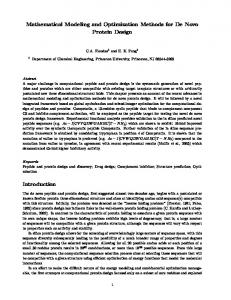
Why convert to clauses? Mainly because this will make it easier to solve relaxations (discussed below). But other approaches are possible. To solve the problem I will not actually need to generate all of the clauses in (10) and (11). I noted earlier that, in general, there can be a very large number of these. But it will be instructive to have a complete list of clauses. Figure 1 shows a branch-and-cut tree for the problem. I will discuss one node at a time.

Root node. I rst solve a relaxation of the problem, but not a linear programming relaxation.

For purposes of illustration I will solve the simplest possible discrete relaxation: I will simply ignore the constraints and obtain the solution x = (x1; x2; x3) = (0; 0; 0), for which the objective function has value 0. After one solves the LP relaxation in branch-and-cut, one can add separating cuts, which are constraints that are not satis ed by the solution of the relaxation. I can do the same here. I will add logic cuts, namely logical clauses from the lists (10) and (11) that are not satis ed by the solution x = (0; 0; 0) of the relaxation. In this case x1 _ x3 and x2 _ x3 are \separating." In general I would look for an ecient \separation algorithm" for nding violated cuts rather than picking them from a complete list, which could be very long. More on this later. Left child. To generate children of the root node I branch on x1. Experience in solving satis ability problems [27] shows that the choice of variable to branch on is extremely important, but I will postpone discussion of \branching rules." The left child is obtained by setting x1 = 0. At this point I can do some logic processing on the clauses obtained so far (only 2 in this case), on the chance that it may allow me to detect inconsistency or x the values of some variables. Here I will apply unit resolution, also called forward chaining. Since x1 is xed to 0, I delete all clauses containing x1 7

Figure 1: Logic-based solution of a small integer programming problem.

min 3x1 + 4x2 + 2x3 s.t. 2x1 ? x2 + x3  1 ?x1 + 3x2 + 5x3  3 Value of relaxation = 0 (x1; x2; x3) = (0; 0; 0) Generate separating cuts:

x1 _ x3 x2 _ x3

x1 = 0 ?

? ?

@ @

? ?

Apply unit resolution: x3 xed to 1; no clauses remain. Relaxation = 2 x = (0; 0; 1) No separating cuts; solution feasible. Backtrack.

x1 = 1

@ @

@

Apply unit resolution: no variables xed, simpli ed problem is

x2 _ x 3

Relaxation = 5 Since 5 > 2, backtrack. No more branching needed.

8

(since they are already satis ed) and delete all occurrences of x1 (since they cannot be true). This leaves,

x3 x2 _ x3

Since the rst clause it is a unit clause (only one literal), it in eect xes x3 to 1, and I can repeat the procedure. I continue in this manner until no unit clauses remain. In this case I delete the second clause because it contains x3 and stop, with no clauses at all remaining. Now I solve a relaxation that takes into account the variables xed so far and the remaining clauses. No clauses remain, but x1 = 0 and x3 = 1 are xed. It is trivial to minimize the objective function subject to these constraints, and I obtain x = (0; 0; 1) as a solution of the relaxation, with objective function value 2. At this point there are no more separating logic cuts; i.e., none of the remaining clauses in (10)-(11) are violated. This means that the solution of the relaxation is feasible, and I have a candidate solution of the problem. I therefore backtrack to the root. Right child. After xing x1 = 1, I again apply unit resolution, which xes no further variables and leaves the one clause x2 _ x3 . To solve the relaxation, I not only x x1 = 1 but bear in mind that at least one of x2 ; x3 must be 1. Thus the rst term of the objective function 3x1 + 4x2 + 2x3 must be 3, and the sum of the last two terms is at least 2 (the smaller of the coecients). So x = (1; 0; 1) solves the relaxation with value 5, which provides a lower bound on the optimal value of the original problem. Since the incumbent solution x = (0; 0; 1) has value 2, which is better than the lower bound 5 obtained at the right child, I can fathom the right child; none of its children can deliver an optimal solution. So the search is over and x = (0; 0; 1) is an optimal solution. The example fails to illustrate what happens when the relaxation is solved with more than one clausal constraint. Suppose for example that I want to minimize (5) subject to two clauses,

x1 _ x2 x2 _ x3

If the clauses were decoupled (i.e., used disjoint sets of variables), the problem could be decomposed. But since they are not, the simplest approach is solve the relaxation separately for each constraint and use the tightest resulting bound. The rst constraint above yields a lower bound of 3 and the second a lower bound of 2. I therefore take 3 to be the value of the relaxation, with x = (1; 0; 0). Although I did not do so here, it may be advantageous to add a constraint 3x1 + 4x2 + 2x3  ; or ? 3x1 ? 4x2 ? 2x3  ? ; (12) that places an upper bound on the objective function. A constraint such as (12) would have no eect on the relaxation, since the objective function is smallest when each xj = 0, which satis es (12) due to the negative coecients. But it may allow the logic processing step to detect inconsistency and thereby prune the search tree. The example of Fig. 1 raises several issues that later sections will examine in more detail. 9

Logic processing. The above algorithm applies unit resolution at each node to simplify the

problem. But unit resolution is an incomplete inference method; it does not always detect when clauses are inconsistent or variables can be xed. I could go to the extreme of using a complete inference method, but it could be slow. The other extreme is to do no processing at all. There are also a number of incomplete methods other than unit resolution. Which is the most eective approach? Branching rule. The choice of which variable to branch on at each node of the search tree is critical. A good branching heuristic should a) simplify the logic processing at successor nodes, and b) provide a tight relaxation at successor nodes. Are these goals incompatible, and what are some good branching rules? Separation algorithm. The above algorithm generates logical clauses that are violated by the current solution of the relaxed problem (i.e., \separating" logic cuts). What is an ecient algorithm for doing this? Deeper cuts. The logic cuts obtained above are analogous to Gomory cuts, in that they are always separating, they consider one constraint at a time, and they do not exploit special problem structure. Integer programming experience shows, however, that one can obtain more eective algorithms by identifying classes of deep cuts, perhaps facet-de ning cuts, that take advantage of problem structure. Can this be done for logic cuts? Is there a logic-based parallel to the theory of facet-de ning cuts? Choice of the relaxation. The relaxation would in general minimize the objective function subject to a) the fact that some variables have been xed and b) some or all of the logic cuts that have been generated. This raises the question: which of the logics cuts should be included in the constraint set of the relaxation? In the above example, they were all included, but one at a time. In general some more complex cuts, particularly those that exploit problem structure, could make the relaxation too hard to solve, even if used one at a time. It may be advantageous to omit them from the relaxation, since they could still be valuable in the logic processing phase, where they would help an incomplete inference method to x more variables. (An incomplete method recognizes only the more explicit implications, and the role of deep logic cuts is to make implicit implications more explicit.) So again, the question arises: which constraints should be included in the relaxation? Solution of the relaxation. A closely related question is obviously, what sort of constraints make the relaxation too hard to solve? How should the relaxation be solved when it is not too hard?

5 A Branch-and-Cut Algorithm I will now state more rigorously the logic-based branch-and-cut algorithm illustrated in the previous section. The algorithm, displayed in Fig. 2 begins with an integer programming problem (9). It may be assumed without loss of generality that c  0, since if cj < 0, xj can be replaced by 10

Figure 2:

Logic-Based Branch-and-Cut Algorithm. Set UB= . Execute ( 0), where = ( End.

1 Branch ;; v;

v

u; : : :; u).

Branch(S ,v,k) If k = 0 then

Procedure

the optimal solution is the best found so far (infeasible if none found); stop. Perform on . If a contradiction is found, return. Perform on . If LB UB, backtrack. Perform on . Branch: Pick a literal containing a variable that occurs in . Perform ( + 1). Perform ( + 1). End.

Unit-Resolve



S

Solve-Relaxation Generate-Cut

S; U

S; U

L

S Branch S [ fLg; v; k Branch S [ fLg; v; k

1 ? xj to obtain a positive coecient. S is the current set of clauses. v is a boolean vector (v1; : : :; vn ), where vj is the value to which xj has been xed; vj = u if xj has not been xed. k is the current level in the search tree. UB is the value of the best solution found so far, and LB is the value of the current relaxation. Unit resolution is simply stated as in Fig. 3. The relaxed problem minimizes the objective function cx subject to a) the variables that have been xed, and b) the logical clauses that have been generated. I will suppose again that the problem is solved separately for each clause C , although I will later indicate cases in which it is easy to solve the problem subject to all clauses simultaneously. I will distinguish two cases: 1. C contains at least one negative literal. In this case the clause is not binding, because an unconstrained optimum would set all the un xed variables to zero (since c  0), which satis es C . So the minimum value BC of cx subject to C and the variables xed so far, as well as the solution x = v C that achieves that value, is given by, X BC = cj vj (13) j vj 6= u

vjC

=

(

11

vj if vj 6= u; 0 if vj = u:

Figure 3:

Unit-Resolve. While S contains a unit

Procedure

do

clause : Pick a unit clause in . Let be the single literal in the unit clause. If = j set j = 1, and if = j set j = 0. Remove from all clauses containing . If contains the unit clause , stop and return with a . Remove from all occurrences of .

L L x

S

S

S

v

L x L

contradiction S

End.

Solve-Relaxation

L

v

L

Figure 4:

Procedure . Let the value of the relaxation be LB= maxC 2S C .  Let the solution of the relaxation be  = C , where End.

v

v

B

C  = argmaxC2S BC .

2. C contains all positive literals. If C = xj1 _ : : : _ xjm , then the solution is, X BC = cj vj + i=1min c ;:::;m ji j vj 6= u

vjC

8 > < vj if vj 6= u; = > 0 if vj = u and j 6= ji ; : 1 if j = ji ;

where i = argmini=1;:::;m cji . The subroutine that solves the relaxation can therefore be stated as in Fig. 4, Finally, the cut generation (separation) routine can be generally stated as in Fig. 5.

6 Logic Processing The entire branch-and-cut algorithm described earlier already contains many elements of a popular satis ability algorithm, the Davis-Putnam-Loveland algorithm [13, 43], which solves problems in clausal form. This algorithm simply applies unit resolution at every node of the search tree, backtracks if it detects inconsistency, stops if all clauses are satis ed, and branches otherwise. But the branch-and-cut algorithm diers not only because of its bounding mechanism but because it adds new clauses at each node. Due to the rapidly improving eciency of pure satis ability algorithms, it may be useful to apply one in the logic processing phase in order to detect inconsistency and x variables when 12

Procedure

Repeat

Generate-Cut.

Figure 5:

as desired: Choose a constraint of that =  violates. there is no such constraint :  Stop; = is a candidate solution. Return after setting UB=LB. Add to one or more clauses that =  violates and that implies.

bx 

If

x v

S

End.

Ax  a

then

x v

x v

bx 

possible. I will rst mention some incomplete satis ability algorithms that could be used here. I will then survey some recent complete methods. In either case I will discuss only algorithms for problems in clausal form, but I will conclude with a discussion of when it might be useful to use disjunctive normal form.

Incomplete methods. The most popular incomplete method is unit resolution. It is easy

to show that unit resolution detects inconsistency if and only if the linear relaxation of the clauses in inequality form is infeasible [6]. Unit resolution is complete if all the clauses are Horn or renamable Horn. A Horn clause is one that contains at most one positive literal (it is de nite if it contains exactly one positive literal). A set of clauses is renamable Horn if they become Horn when some set of zero or more variables xj are replaced with their complements xj in every occurrence. The running time of unit resolution is quadratic in the number of literals. But if the clauses are all Horn, it suces to eliminate only positive unit clauses, since once this procedure is nished, all the remaining clauses can be satis ed by setting the remaining variables to false. This leads to the linear-time algorithm of Dowling and Gallier [14] for Horn clauses. Thus a method somewhat weaker but faster than unit resolution is to apply unit resolution to the Horn relaxation of the clause set, which is simply the subset of all Horn clauses in the set. A slight strengthening of unit resolution is more eective at xing variables. Namely, for each xj , rst temporarily x xj to true and perform the unit resolution procedure, and then x xj to false and do the same. If the former yields a contradiction, xj should be xed to true, and similarly for the latter. It follows from a theorem in [30] that this procedure obtains a cut of the form xj  1 or ?xj  ?1 if and only if it is a rank 1 cutting plane in Chvatal's sense [11]. There are also a number of heuristics for the satis ability problem [51, 16, 24, 49]. Complete methods. Some of the new methods are based on integer programming. Following early work by Blair, Jeroslow and Lowe [6] and Williams [55], Hooker and Fedjki [28, 33] designed a branch-and-cut algorithm based on a theoretical result in [30]. Harche and 13

Thompson [27] solve an integer programming model with a column subtraction procedure on the simplex tableau for the linear relaxation of the problem. This approach seems one of the most robust. Other mathematical programming approaches include the interior point method of Kamath, Karmarkar, Ramakrishnan and Resende [41, 42] and a linear complementarity approach of Patrizi and Spera [45, 52]. The classical Davis-Putnam-Loveland (DPL) procedure [13, 43], which is a straightforward tree search that performs unit resolution at each node, is competitive with more recent methods when properly implemented. Jeroslow and Wang [40] found an ecient implementation by replacing depth- rst traversal with something more complicated, but it turns out that its eciency is actually due to their branching rule [27]. Branching rules have been studied by Hooker and Vinay [34], Crawford [12] and Dubois et al. [15]. The use of unit resolution at each node if eect solves a relaxation of the problem at that node. The relaxation can be strengthened by generating more resolvents (Billionnet and Sutter [5]) or checking for \local inconsistency" (Freeman [17]). One can also use a weaker relaxation; Gallo and Urbani [19] used a Horn relaxation and Jaumard et al. [37] used Horn and 2-SAT relaxations in combination with tabu search. Gallo and Pretolani [18, 46] used directed hypergraphs to design one of the most ecient algorithms now available. Truemper [53, 54] drew heavily on ideas of combinatorial optimization in his decomposition approach, which generates a solution program while solving one problem that can be used to solve similar problems rapidly. A satis ability problem can always be expressed as a problem of checking whether a logic circuit has the same output for every input. In this form it can be solved with binary decision diagrams [1, 7] or an approach of Hooker and Yan [35] based on Benders decomposition. Results from graph theory have been used to solve certain classes of inference problems in propositional logic [21, 25, 26]. Many of the above algorithms can be modi ed to update a solution rapidly after a clause is added to the problem. Hooker [32] showed how to do this for the Davis-PutnamLoveland algorithm. For more complete surveys of satis ability algorithms, see [9, 10, 27, 29]. Disjunctive normal form. When adding cuts it is most natural to express logical constraints in conjunctive form, which is a conjunction of clauses or other convenient units. When new cuts are added, one simply conjoins more terms. But in some contexts disjunctive form may be advantageous, particularly because it allows one to see immediately which variables are xed. A formula is in disjunctive normal form (DNF) when it is a disjunction of terms, which are conjunctions of literals. The following formula is in DNF: (x1 ^ x2 ) _ (x2 ^ x3) _ (x2 ^ x3 ^ x4): (14) A conjunction of clauses is in conjunctive normal form (CNF). There is a simply duality between DNF and CNF, in that a formula in DNF is equivalent to the negation of a 14

formula in CNF that is obtained by interchanging ^ and _ and negating every literal in the DNF formula. For instance, (14) is equivalent to the negation of, (x1 _ x2 ) ^ (x2 _ x3) ^ (x2 _ x3 _ x4):

(15)

This follows from De Morgan's Law and distribution laws in elementary logic. The duality idea is relevant to the issue of xing variables. Note that the literal x2 occurs in every clause of (15). This means that the unit clause x2 implies (15). In fact a literal L implies a CNF formula F if and only if L appears in every clause of F ,3 but this fact is not particularly useful. However, it becomes useful in the dual: L is implied by a DNF formula F if and only if L occurs in every term of F . So if the logical constraints are in the form of a single DNF formula, I can tell at a glance which variables are xed.

7 Branching Rules In Davis-Putnam type satis ability algorithms, it is critically important to use an intelligent branching rule to choose which variable to x at each node of the search tree [27]. A good branching rule can improve the speed of an algorithm by several orders of magnitude. Since a logic-based branch-and-cut algorithm is similar to Davis-Putnam algorithms, one can expect the branching rule to be important here as well. The main objective of a branching rule is to avoid generating a large tree. In a DavisPutnam setting, this is done by a) nding a satisfying valuation quickly if the problem is satis able, or b) backtracking as soon as possible if the problem is unsatis able. In a branchand-cut algorithm there is another factor, the strength and value of the relaxation that results from xing a variable. Since importance of the second factor is as far as I know poorly understood, I will focus on the rst. Also there is reason to believe that a branching rule that is good for Davis-Putnam algorithms would tend to result in tight relaxations, as I will explain shortly. A widely used branching rule is that proposed by Jeroslow and Wang [40]. It applies only to problems in clausal form. I will say that to branch on a literal L at a given node is to x L to true rst; when and if one backtracks to the node, one obtains the second branch by setting L to false. If S is the set of clauses at the current node, The Jeroslow-Wang rule instructs one to branch on the literal L that maximizes X ?len(C ) J (L) = 2 ; C 2S L2C

where len(C ) is the number of literals in C . So the rule tends to branch on a literal that occurs in many short clauses. Note that if L 2 C , then C will be deleted from the problem when L is xed to true. The rationale for the rule is that since 2?len(C ) is the probability that a random truth valuation falsi es C , it branches to a subproblem that excludes clauses that are more likely to 3 I assume here that a given variable appears at most one in any given clause.

15

be falsi ed by a random truth assignment. In other words, it branches to a subproblem that is easier to satisfy. This presumably allows one to nd a satisfying solution with less backtracking. But Hooker and Vinay [34] nd a number of problems with this rationale. One is that it does not explain the good performance of the rule on unsatis able problems. Another is that when estimating the probability of satisfaction, one should take into account the fact that L will be removed from clauses containing it. This results in the rule that L should maximize

J (L) ? J (L); which performs very poorly. Rules that more accurately estimate the probability of satisfaction are even worse. Hooker and Vinay show evidence that the Jeroslow-Wang rule is best explained as one that results in the creation a large number of unit clauses during unit resolution, which in turn simpli es the problem. This same rationale dictates a \2-sided" Jeroslow-Wang rule that is substantially better than the 1-sided rule; namely, maximize

J (L) + J (L): Since Jeroslow-Wang-type rules tend to result in more unit clauses, they x more variables at a node and are therefore likely to strengthen the relaxation. Another rule that exhibits good performance [34, 27, 19] is shortest positive clause branching. That is, pick the shortest clause xj1 _ : : : _ xjm in S that contains all positive clauses, and generate m branches. In the rst branch, set xj1 = 1. In the second, set xj1 = 0 and xj2 = 1. In the third, set xj1 = xj2 = 0 and xj3 = 1, and so on. Note that this is the same as branching on variables in the order xj1 ; xj2 ; etc. That is, the root has children created by setting xj1 = 1 and xj1 = 0, respectively. The negative child (in which xj1 = 0) has children in which xj2 = 1 and xj2 = 0. The negative child is similarly expanded, and so on. So the clause branching rule is essentially a variable branching rule that branches on a variable in the shortest positive clause. Since this approximates the JeroslowWang criterion J (L) (which favors literals in short clauses), it is not surprising that it works well. Also, by picking an all-positive clause it also exploits the fact that there is no point in branching on a variable that never occurs in an all-positive clause, because all the clauses containing that variable can be satis ed simply by setting all their variables to false. In fact this feature can be added to a Jeroslow-Wang-type rule by branching only on variables that occur in some all-positive clause, often with a resulting improvement in performance.

8 Separation Algorithms In this section I will discuss how to generate separating logic cuts that belong to certain simple classes. As I noted earlier, these cuts are analogous to the Gomory cuts of classical integer programming. I will rst consider cuts that are logical clauses. Suppose I want to generate separating clausal cuts for the inequality constraint, 3x1 ? 2x3 + 4x4 ? x6 + 2x8 + 3x9  9: 16

I will rst make all the coecients positive by replacing each xj with yj if its coecient is nonnegative and otherwise with 1 ? yj . 3y1 + 2y3 + 4y4 + y6 + 2y8 + 3y9  12:

(16)

I will suppose that the current solution of the relaxed problem is y = (y1 ; : : :; y9) = w = (1; 1; 1; 1; 0; 0; 0; 0; 0). I want to nd separating clausal cuts; i.e., clauses implied by (16) that y = w fails to satisfy. It is easy to show that since all the coecients of (16) are nonnegative, any clause that (16) implies is absorbed by some implied clause that has only positive literals. So I need only consider cuts with all positive literals. Obviously none of the separating cuts contain y1 ; y3 or y4 , since any such cut is satis ed by y = w . So I want to generate positive clauses that contain no literals other than y6 ; y8; y9 and that (16) implies. We would expect that the cuts containing these three literals would be only a small fraction of those containing any of the six, since there are 26 subsets of all six and only 23 subsets of the last three. In general, the separating cuts should comprise only a small fraction of all cuts. To generate the cuts containing y6 ; y8; y9 I can use a straightforward enumerative algorithm similar to that of Granot and Hammer [22]. In order to generate the strongest cuts rst, I will order the terms by decreasing coecient size: 3yj1 + 2yj2 + yj3 : I rst check whether a clause containing only the rst term yj1 is a cut. It is not; the remaining terms of the inequality can sum to a number as large as 12. I therefore try adding yj2 :

yj1 _ yj2 ; and obtain a cut. If I had not obtained a cut, I would have added a third literal. Next I try adding yj3 :

yj1 _ yj3 ; and obtain a second cut. I continue by trying yj2 alone (which is not a cut), and so forth, but obtain no further cuts. In general I want to nd separating cuts implied by an inequality ax  . I will Let (  0; yj = 1xj? x ifif aaj < j 0; (  j  0; wj = 1vj? v  ifif aaj < j 0; Xj =? aj j aj < 0

where v  is the solution of the current relaxation. I will assume that jaj1 j; : : :; jajm j are arranged in order of decreasing size. I may also want to generate only cuts belonging to some subclass P of clauses, such as positive clauses (if I am solving the relaxed problem subject to one clause 17

Figure 6:

Separation Algorithm for Clauses. Perform ( 0). End.

Cut ;;

Cut(T; k). If Wi2PT yji 2 P then: If i62T jaji j < thenW

Procedure

Generate the cut

End.

i2T yji .

Else For i = k + 1; : : :; n do: If wji = 0 then perform Cut(T [ fig; i).

at a time4 ) or Horn clauses (if I am solving it subject to all the clauses simultaneously). The algorithm appears in Fig. 6. If there are a large number of separating cuts, the algorithm can be terminated prematurely after generating K cuts, and it will have generated the K strongest (i.e., shortest) cuts. It is also possible to generate separating cuts that are stronger than clauses. Barth [3], for instance, shows how to generate separating extended clauses. These have the form,

aj1 xj1 + : : : + ajm xjm  k;

(17)

where each aji 2 f1; ?1g. Stronger cuts can be fewer in number, and Barth found that (1) is equivalent to 4282 extended clauses, as compared with 117520 ordinary clauses.

9 Solving the Relaxation I will rst discuss minimizing the objective function cx, for c  0, subject to a single logical formula. Since I can ignore the variables xj whose values are xed, I will assume they have coecient zero. I discussed earlier how to minimize cx subject to a clause C = xj1 _ : : : _ xjm , which I can assume to contain all positive literals, since otherwise it is not binding (because c  0). Namely, the minimum is simply the smallest cji for i 2 f1; : : :; mg. It is also easy to minimize cx subject to an extended clause (17). In fact I can assume that each aji = 1, since if aji = ?1 I can drop aji xji from the sum and obtain a constraint that has the same eect. The minimum value of cx is simply the sum of the k smallest cji 's for i 2 f1; : : :; mg. 4 Note, however, that if only positive separating cuts are generated, inconsistency can never be detected. If the constraints include a bound on the objective function, then cut generation should not be restricted to positive clauses, since otherwise the constraint that imposes the bound would serve no function because it does not imply any positive clauses.

18

It more interesting, however, to consider when it is easy to minimize cx subject to a set of logical formulas. One particularly nice case is that in which the set of boolean vectors satisfying the formulas has a minimum element. That is, some feasible x has the property that x  x0 for every feasible x0. In this case the minimum element minimizes cx for any set of (nonnegative) coecients. As it happens there is a well-known class of logical formulas that has this property: Horn clauses. In fact the minimum element satisfying a set of Horn clauses can be obtained in linear time by applying a Dowling-Gallier algorithm [14]. It is also easy to generate a set of separating Horn cuts. Another class of easy problems are those that can be solved by dynamic programming. Suppose the variables can be ordered xj1 ; : : :; xjn so that the feasibility of xji depends only on the value of xji?1 . That is, for a xed boolean pair (tji?1 ; tji ), (xj1 ; : : :; xjn ) = (tj1 ; : : :; tjn ) is feasible for one boolean value of t = (tj1 ; : : :; tji?2 ; tji+1 ; : : :tjn ) if and only if it is feasible for all boolean values of t. In this case the minimum can be found recursively by calculating, fi (xji ) = min fcji + fi+1 (xji+1 )g; xji+1 2Di+1 (xji )

where Di+1(xji ) is the set of feasible values of xji+1 given xji . The boundary condition is f0 (0) = f0(1) = 0 and the minimum value is minff1 (0); f1(1)g.

A set of formulas has this property if its dependency graph is a chain (or set of chains). The dependency graph is constructed by associating a vertex with every variable xj , and connecting xj and xk with an edge if they occur in the same constraint. More generally, if the dependency graph is a partial k-tree [2], then cx can be minimized using nonserial dynamic programming [4, 8] in time that is proportional to 2k . Thus when k is small, the relaxed problem can be quickly solved subject to all the constraints simultaneously.

10 Example of Logic Cuts Experience in combinatorial optimization has shown that one must often take advantage of problem structure before the problem can be solved. In other words, general-purpose methods are often ineective. One way to exploit structure in integer programming is to identify strong cuts for a particular class of problems, such as cuts that de ne facets of the convex hull of integer solutions. An analogous approach can be used in logic-based methods. In fact, logic-based methods should provide more opportunities to exploit structure. The identi cation of strong polyhedral cuts requires that one analyze the convex hull, and this can be a dicult task even for relatively simple problems. The identi cation of logic cuts, however, need not involve polyhedral issues. One may be able to state useful logical relationships among integer variables in problems whose convex hull is far too complex to analyze. In fact, facet-de ning cuts are often discovered even in simple problems by rst identifying logical relationships and then writing inequalities to capture the relationships. Furthermore, logic cuts need not be discovered through an analysis of the abstract mathematical structure of an integer programming model. They can be found by analyzing the problem that the model tries to capture, where the concreteness of the situation may be more suggestive. I will give a simple example of how logic cuts may be inferred from a concrete understanding of the problem. I will supply further examples in my later discussion of mixed integer 19

Figure 7: A political districting problem. 12 hhhhhh

( 8 (( 10

 @

 

 A  @  A @  A @ 

6

 

B @  11 hhhhhh B 9  25 20 PP ? A

B 4  C PP A

B E  CC ?? 1  T A

" B E  TT  " 13 hhhh 3 hh  17 "   hhh E " ? 7  A 2  ?  C " A ?? ? " C 16  CC " 19 XXXX ? C " "  B C 21 hhh  h 15 C  B # B 5Q B # B ? # Q B # B ? Q B Q

 30 

18 Q

 Q QQ  

22

24

c  cc 

23

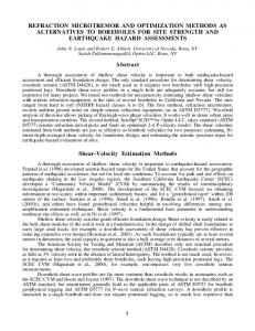
programming. Suppose 25 geographic regions are to be grouped into political districts. In the graph in Fig. 7, vertices correspond to regions and edges connect adjacent regions. For convenience, let each district be indexed by its population. The total population of 341 is to be divided into six contiguous districts of as nearly equal population as possible. For the sake of illustration I will express the objective as one of minimizing the maximum district size, subject to the constraint that every region belong to exactly one contiguous district. This is a very early application not only of integer programming but of what was essentially a logic-based method (Gar nkel and Nemhauser [20]). One IP formulation of the would go as follows. Let ( region i assigned to district j xij = 10 ifotherwise ; pi = population of region i. Then the model is, min z X s.t. z  pi xij ; j = 1; : : :; 6; i

20

(18)

6 X

j =1

xij = 1; all i

contiguity constraints all xij 2 f0; 1g:

There are various (awkward) ways to formulate contiguity constraints, but there is really no point in writing a formulation. I will branch in such a way that contiguity is maintained. To reduce the search I will place an upper bound on the value of the objective function. Since the average district population 56.8 is a lower bound on the largest district population, I will require every district's population to be less than a number near 56.8, say 60. X pi xij  60; j = 1; : : :; 6; (19) i

It follows that every district population must be at least 41. Initially a practitioner familiar with the problem can observe that certain population centers cannot lie in the same district. For instance, regions 25 and 30 (circled in Fig. 7) cannot lie in the same district because every connecting path contains regions whose populations sum to more than 60. Similarly, region 20 cannot lie in the same district as either 25 or 30. We can therefore enforce x25;1 = x30;2 = x20;3 = 1 as initial logic cuts. To enforce contiguity, I allow myself to x xij = 1 only if a) region i is adjacent to a region assigned to district j , or b) no region has been assigned to district j . It is easy to identify some separating cuts at each node of the search tree. Suppose for instance that regions 4, 25, 9 and 12 have been assigned to district 1. Then regions 8 and 10 form an \enclave," which is Gar nkel and Nemhauser's term for a contiguous set of regions, having a combined population too small for a district, that are isolated by assigned regions.5 Each member of the enclave must be assigned to one of the adjacent districts. Since district 1 is the only adjacent district, I have a logic cut,

x8;1 = x10;1 = 1: Consider an example of an enclave adjacent to two districts. Suppose that nodes 8, 25 and 17 have been assigned to district 1 (circles in Fig. 8), and nodes 18, 5 and 19 have been assigned to district 3 (squares). Then nodes 4, 7 and 16 form an enclave. First of all I have the enclave cuts I discussed earlier.

x4;1 _ x4;3 x7;1 _ x7;3 x16;1 _ x16;3

When there are two or more adjacent districts, the enclave cuts are rather weak. They merely prevent me from starting a new district in the enclave. But they can tighten the 5 Actually they also regard the regions in an enclave as having been assigned to districts.

21

Figure 8: Illustration of an enclave.

 10 8   25   17 

12 hhhhhh

(((

 @

 A  @  A @  A @ 

6

B @   h 11 hhhhh B 9  20 PP

B ? A 4  C PP

? A B E 1 CC ?  T  A "

B E   T " 13 hhhh 3 hh T   "   hhh E " ? 7  A 2   ? C  " A ?? " ? C 16  CC " 19 XXXX ? CC " "  B hhh C 21  h C 15  B # B 5Q B # B ? # Q BB ? # Q B Q

18 Q

 Q QQ  

22

30

24

c  cc 

23

22

Table 1: Populations of districts 1 and 3 and their enclave. Nodes Population District 1 8, 25, 17 50 District 2 18, 5, 19 42 Enclave 4, 7, 16 27 Total 119 relaxation I might solve to get a lower bound on the population of the largest district. I know that the enclave population must somehow be distributed to districts 1 and 3 (Table 10). So I can distribute their total population 119 equally between the districts to obtain a lower bound of 59.5 on the population of districts 1 and 3. This improves the previous lower bound of 56.8 on the population of the largest district (i.e., the average district population). It is easy to see how to write the separation algorithm for enclave cuts. Initially, give a white label to an arbitrary unassigned node, and regard the rest of the nodes as unlabeled. Then do the following as long as possible. Pick any unassigned node with a white label, make its label red, and give all adjacent nodes white labels. When the algorithm has nished, make a list of all districts containing white-labeled nodes. If the total population of the red-labeled nodes is less than the minimum district population, each red-labeled node must be assigned to some district on the list. The whole procedure is run repeatedly, each time beginning with a node that was not labeled in any previous runs. Each run generates a set of cuts. One can identify an number of other cuts that were not used by Gar nkel and Nemhauser. Note in Fig. 8, for instance, that either node 4 is assigned to district 1, or else nothing from the enclave is assigned to district 1: x4;1 _ (x4;3 ^ x7;3 ^ x16;3): Since the latter alternative pushes the district 3 population over 60, this cut in eect xes x4;1 = 1. Similarly, either at least one of nodes 7 and 17 is assigned to district 3, or else nothing in the enclave is. x7;3 _ x16;3 _ (x4;1 ^ x7;1 ^ x16;1): Again the latter alternative is infeasible, so that in eect I have x7;3 _ x4;3. In the present case this sort of cut does not improve the relaxation, since neither the addition of node 4 to district 1, the addition of 7 to 3, nor of 16 to 3 raises the population of a district above the previous bound of 59.5. But in other cases it could improve the bound. In general such a cut can be obtained by considering the set S of all nodes in the enclave that are adjacent to one of the districts (say, j ) bordering the enclave. Then either a) one of the nodes in S must be assigned to j , or b) all of the nodes in the enclave must be assigned to bordering districts other than j .

11 Strong Cuts In this section I will de ne the strongest type of logic cut, namely a prime cut. It is the logical counterpart of a facet-de ning cut, the strongest polyhedral cut. Logic cuts in practice need 23

not be prime and often are not, but one can gain some understanding of what a \strong" logic cut is by de ning the strongest type of logic cut. Recall rst that a facet-de ning cut for an integer programming problem (9) is an inequality bx  that de nes a facet of the convex hull of feasible solutions of (9). Thus if the convex hull has dimension d, bx  de nes a facet if and only if it is a valid cut and there are anely independent points y1 ; : : :; yd such that Ayj  a and byj = for j = 1; : : :; d. To de ne the strongest possible logic cut, I will rst review the notion of a prime implication de ned by Quine 50 years ago [47, 48]. Given a set S of logical clauses, clause C is a prime implication of S if S implies C but implies no other clause that implies C . For instance, the prime implications of the set

are:

x1 _ x2 x1 _ x2 x3 _ x4 x3 _ x5

(20)

x1 x3 _ x4 x3 _ x5 x4 _ x5

(21)

Every clause implied by (20) is implied by a clause in (21). Some prime implications can be redundant of the others, as is the fourth clause in (21). Nonetheless a prime implication is in some sense a strongest possible implication.6 This idea is easily generalized to 0-1 linear inequalities, which are after all logical propositions. I will say that a logical formula F is a prime cut of Ax  a with respect to a class T of formulas if F is equivalent to any formula in F that is implied by Ax  a and implies F . If F is a 0-1 inequality and T a class of 0-1 inequalities, I will say that F is a prime inequality for Ax  a with respect to T . It is important to realize that a single prime cut may take the form of many equivalent but dierent inequalities that bear no obvious relation to one another. For instance, one prime cut of the inequalities, x1 + 2x2 + x3  2 x1 ? x2  0; can be variously written, x2 + x 3  1 3x2 + 5x3  2 50x2 + x3  1 etc. Although prime cuts and facet-de ning cuts are analogous concepts, there is no simple relation between them. A prime cut can even strictly imply a facet-de ning cut, as the following 6 Quine actually de ned the dual notion, a prime implicant for a formula in disjunctive normal form, which

is a term that implies the formula but that is implied by no other term that implies the formula. A prime implication is also called a prime implicate.

24

Figure 9: Illustration of a prime logic cut.

example shows. Consider the constraint set,

x1 + x2  1 x2 + x3  1

(22) (23)

Figure 9 shows the convex hull of the integer solutions, whose nonelementary facets are de ned by the inequalities (22)-(23). The following is a prime cut for (22)-(23).

x1 + 2x2 + x3  2:

(24)

It de nes a cutting plane shown in Fig. 9. Note that it is equivalent to neither facet-de ning inequality and in fact strictly implies both. For instance, every 0-1 point that satis es (24) satis es (23), and one point|namely, (x1 ; x2; x3) = (1; 0; 0)|satis es (22) but does not satisfy (24). On the other hand, since any valid inequality is dominated by a positive linear combination of facet-de ning inequalities, this is true in particular of a prime inequality. For instance, the prime cut (24) is simply the sum of the facet-de ning inequalities (22) and (23). 25

The role of prime cuts in integer programming is parallel to that of facet-de ning cuts. If the constraint set Ax  a of an IP (9) contains the facet-de ning inequalities for the convex hull of feasible points, then the IP can be solved in its LP relaxation|or as the dual of the LP relaxation. That is, if is the optimal value of the objective function cx, then cx  is dominated by some nonnegative linear combination of the constraints. Similarly, if Ax  a contains all its prime cuts (up to equivalence), the IP can be solved as a series of 0-1 knapsack problems, one for each constraint. For in this case if is again the optimal value, cx  is implied by some single constraint. (Recall that checking for implication between inequalities is a 0-1 knapsack problem). More precisely, Theorem 3 Let be the optimal value of the integer programming problem (9). Then if cx  belongs to a class T of inequalities with respect to which Ax  a contains all its prime cuts (up to equivalence), cx  is implied by one of the inequalities in Ax  a. Logic cuts may seem less eective than polyhedral cuts because they reduce an IP to another NP-hard problem|a series of knapsack problems|whereas polyhedral cuts reduce an IP to an LP. But the LP is in general exponentially large if it contains all facet-de ning cuts. In practice, one never generates more than a small fraction of facet-de ning or prime cuts. The important issue is how eectively a few well-chosen cuts reduce the size of the search tree. There is no reason to believe a priori that logic cuts are less eective in general than polyhedral cuts.

12 Generation of Prime Cuts A fundamental result of integer programming, due to Chvatal [11], says that a nite procedure generates all facet de ning cuts for a 0-1 system Ax  a. A rank 1 cut for Ax  a is any inequality obtained by rounding up noninteger coecients and right-hand sides in a nonnegative linear combination uT Ax  uT a (u  0) of the inequalities. If S is the set of all cuts of Ax  a of rank less than or equal to k, then one can obtain all cuts of rank less than or equal to k + 1 by adding to S its rank 1 cuts. Chvatal proved the following. Theorem 4 If the solution set of a 0-1 system Ax  a is nonempty and bounded, then any valid cut is dominated by a rank k cut for some nite k. In particular, any facet-de ning cut is dominated by some rank k cut. A parallel result can be proved for logic-based programming [31]. Rather than taking all rank 1 cuts, it uses two particular types of rank 1 cuts: resolvents (discussed earlier) and diagonal sums. Two clauses have a resolvent when there is exactly one variable xj that appears positively in one and negatively in the other. The resolvent contains all the literals in either clause except xj and xj . For instance, the third clause below is the resolvent of the rst two.

x1 _ x2 _ x3 x1 _ x2 _ x4 x2 _ x3 _ x4 26

Quine [47, 48] showed that repeated resolutions generate all prime impolications of a set of clauses. To see that resolvents are rank 1 cuts, write the above clauses as the rst, second and fth inequalities below. x1 + x 2 + x3 1 ?x1 + x2 ? x4  ?1 x3 0 (25) ? x4  ?1 x2 + x3 ? x4  0 The resolvent can be obtained by a) taking a linear combination of the rst two inequalities and the two bounds (inequalities 3 and 4 above), where each is given a weight of 1/2, and b) rounding up the right-hand side. The resolvent is therefore a rank 1 cut of the parent inequalities and trivial bounds of the form 0  xj  1. To illustrate a diagonal sum, I will consider the following inequalities.

x1 + 5x2 + 3x3 + x4  4 2x1 + 4x2 + 3x3 + x4  4 2x1 + 5x2 + 2x3 + x4  4 2x1 + 5x2 + 3x3 4 2x1 + 5x2 + 3x3 + x4  5 Note that each of the rst four inequalities is the same except that the diagonal coecients are reduced by one. The fth inequality is their diagonal sum. It is a rank 1 cut because it can be obtained by taking a linear combination of the four inequalities with respective weights 2/10, 5/10, 3/10 and 1/10 and rounding up the right-hand side. Recall that X n(a) = aj : j aj < 0

A feasible inequality ax  + n(a) is the diagonal sum of the inequalities ai x  ? 1 + n(ai ) for i 2 J  f1; : : :; ng = N when aj 6= 0 for all j 2 J , aj = 0 for all j 2 N n J , and 8 > < aj ? 1 if aj > 0; aij = > aj + 1 if aj < 0; : aj otherwise: To verify that ax  + n(aP) is a rank 1 cut (when n  2), assign each ai x  ? 1+ n(ai ) weight jaij=(W ? 1), where W = j jaj j. The weighted sum of the inequalities aix  ? 1 + n(ai) is ax  ( ? 1)W=(W ? 1)+ n(a). Since feasibility implies W  , I have ? 1 < ( ? 1)W=(W ? 1)  , so that I get the desired ax  + n(a) after rounding up the right-hand side. The algorithm in Fig. 10 generates prime inequalities for Ax  a with respect to a class T of inequalities. The rank of a logic cut can be de ned in analogy with that of polyhedral cuts. Let set T of inequalities be monotone when T contains all clausal inequalities, and for any given inequality ax  + n(a) in T , T contains all inequalities a0x  0 + n(a0 ) such that ja0j  jaj and 0  0  . The following theorem is proved in [31]. 27

Figure 10:

Algorithm for Generating Prime Cuts.

Ax  b

S

Let contain the inequalities in . Turn off the termination flag. the termination flag is off : Turn on the termination flag. If possible, find clausal inequalities and in that have a resolvent that no inequality in implies, such that and are each implied by some inequality in this is possible : Turn off the termination flag. Remove from all inequalities that implies, and add to . If possible, find inequalities 1 m in that have a diagonal sum in that no inequality in implies, such that 1 m are each implied by some inequality in . this is possible : Turn off the termination flag. Remove from all inequalities that implies, and add to .

While

do

S

R

S

If

C

C

then

S

R

I

S

If

S

then

S

I

28

S

D

D

S

R

I ; : : :; I T

T

I ; : : :; I S I

Theorem 5 If the above algorithm is applied to a feasible 0-1 system Ax  a so as to generate set S of inequalities, and T is a monotone set of inequalities, then every prime cut for Ax  a

with respect to T is equivalent to some inequality in S .

13 Matching Problems Matching problems provide an instructive illustration of logic cuts.7 A matching problem is de ned on an undirected graph (V; E ) for which each edge in E is given a weight. The edges connect vertices that may be matched or paired, and a matching pairs some or all of the vertices. A matching can therefore be regarded as a set of edges, at most one of which touches any given vertex. The weighted matching problem is to nd a maximum weight matching; i.e., matching that maximizes the total weight of the edges used in the matching. The matching problem can be written, X max xe (26) e2E X s.t. xe  1; for v 2 V (27) e2(v) xe 2 f0; 1g;

e 2 E;

where  (v ) is the set of edges incident to v . xe is 1 when e is part of the matching and 0 otherwise. The convex hull of possible matchings has a particularly simple description. It is based on the fact that a matching for a graph (U; E ) with an odd number of vertices can have at most jU j edges. So the following odd set constraints are valid: 2 X xe  jU2 j ; all U  V with jU j  3 and odd, (28) e2E (U ) where E (U ) contains the edges in the subgraph of (V; E ) induced by U . In fact (27)-(28) de ne the convex hull of matchings. It is an interesting exercise to obtain odd set constraints as logic cuts from (27) using the algorithm in Fig. 10. First reverse the sense of the matching constraints (27) and odd set constraints (28) by replacing variables xe with ye = 1 ? xe , so that ye = 1 when edge e is absent from the matching. X ye  j(v)j ? 1; for v 2 V (29) e2(v)

X

e2E (U )

ye  jE (U )j? jU2 j ; all U  V with jU j  3 and odd.

7 This section represents joint work with Ajai Kapoor.

29

(30)

Figure 11: A small matching problem.

y1

f

? ?

@

? ?

? ?

?

@ @ y5 @ @ @ @

f

y2

f

@ @ @

y4

y3

@ @

@ @

f

f

Next consider an example. The matching constraints for the graph in Fig. 11 are: y1 + y 2 + 1 y2 + y 3 1 y3 + y 4 1 y1 + y4 + y5  2

(31)

The only odd set constraint other than those already listed in (31) is, y1 + y2 + y3 + y4 + y5  3: (32) This constraint is a rank 2 logic cut. It is the result of a diagonal sum of the inequalities, y2 + y 3 + y 4 + y 5  2 y1 + y3 + y4 + y5  2 (33) y1 + y 2 + y4 + y5  2 y1 + y 2 + y 3 + y5  2 y1 + y 2 + y 3 + y 4  2: The rst premise of this sum is itself the result of a diagonal sum of the inequalities, y3 + y 4 + y 5  1 y2 + y4 + y5  1 (34) y2 + y 3 + y5  1 y2 + y 3 + y 4  1: Note that each inequality of (34) is implied by one of the inequalities of (31). The rst is implied by y3 + y4  1. The second is implied by y1 + y4 + y5  2. The last two are implied by y2 + y3  1. The other premises in (33) can be similarly obtained, so that (34) is indeed a rank 2 logic cut. 30

Figure 12: An even smaller matching problem.

i

y1

i

y2

i

y3

i

In general any odd set constraint (30) can be obtained by a similar hierarchy of diagonal sums. (30) is the diagonal sum of jE (U )j inequalities with degree jE (U )j? jU2 j ? 1, which in turn are diagonal sums of inequalities with degree jE (U )j? jU2 j ? 2, and so on down to inequalities with degree 1. It is necessary only to make sure that each of the degree 1 inequalities is implied by one of the matching constraints, as are (32) in the example. But the degree 1 inequalities have the form, X ye  1; (35) e2E 0

where jE 0j = jE (U )j ? (jE (U )j ? jU2 j ? 1) = jU2 j + 1. The inequalities (35) are clearly valid, because it is impossible for jU2 j + 1 edges to belong to a matching on jU j vertices; at least two edges e1 ; e2 must be incident to the same vertex v . In fact, the matching constraint (29) for vertex v implies (35). This is because (29) can be reduced to X ye  1; (36) e2fe1 ;e2 g

since  (v ) contains j (v )j ? 2 edges other than e1 ; e2. But (36) absorbs (35).

Theorem 6 An odd set constraint (29) for a matching problem is a logic cut of rank at most jE (U )j ? jU j ? 1. 2

Odd set constraints are not in general prime cuts. They are strictly implied, for instance, by another well-known class of cuts|augmenting path cuts. In Section 11, for instance, I pointed out that although y1 + y2  1 and y2 + y3  1 de ne facets of the convex hull of their satisfaction set, they are strictly implied by the logic cut y1 + 2y2 + y3 . This is in fact an augmenting path cut for the simple network of Fig. 12. It says that either the middle segment or the two end segments may belong to a matching, but not both. In general a path of odd length whose edges correspond to yj1 ; : : :; yjm de nes an augmenting path cut, m?1 y + m+1 y + m?1 y + : : : + m+1 y m?1 j1 j2 j3 jm?1 + 2 yjm 2 2 2 2



m?1)(m+1) ;

(

2

which says that if the (m +1)=2 odd segments belong to a matching, then none of the (m ? 1)=2 even segments may belong to it, and vice-versa. 31

14 The Logic of Mixed Integer Programming From a logical point of view, mixed integer programming generalizes integer programming by replacing points with polyhedra. Whereas each solution of an IP is associated with a point, each feasible assignment of 0-1 values to an MIP is associated with a polyhedron. This requires some explanation. Consider a general MIP, min cx + dy (37) s.t. Ax + By  a yj 2 f0; 1g; j = 1; : : :; n; where x is a vector of m continuous variables and y a vector of n 0-1 variables. I will say that a 0-1 vector y is feasible for (37) if (x; y ) is feasible in (37) for some real x. Each feasible 0-1 value of y is associated with a polyhedron in x-space, namely the set of points satisfying (37) when y is so xed. This is a polyhedron because for any xed y , the constraints in (37) becomes linear inequalities in x. The feasible region for (37) can be regarded as the union of all the polyhedra corresponding to feasible values of y . The limiting case of pure 0-1 programming occurs when (37) contains no continuous variables. Here a feasible y is associated with a point, namely the entire 0-dimensional x-space. From this perspective, the point associated with a feasible solution y of an IP is not the point y in n-dimensional space; it is the point 0 in 0-dimensional space. Thus every feasible solution of a 0-1 problem is associated with the same point. In essence the feasibility problem posed by an MIP consists of a set S of logical propositions involving the 0-1 variables yj and a mapping  that assigns a polyhedron to every y satisfying S . I will call this a mixed integer feasibility problem in logical form. The feasible set for this problem is the union of (y ) over all y satisfying S , and the problem is infeasible when this union is empty. In the special case of pure 0-1 programming, (y ) = f0g for all y , and the problem is feasible when at least one y satis es the set S of 0-1 constraints. Thus a mixed integer optimization problem can be written, min cx + dy (38) s.t. y 2 Y[ x 2 (y); y2Y

where Y is the set of 0-1 points satisfying S . The constraints are normally expressed by embedding both x and y in a single constraint set, namely that of an MIP (37). But the problem need not be expressed in this fashion. In fact it is in the spirit of logic-based optimization to treat the problem of nding feasible y 's as a logic problem. For a given feasible y , the problem of checking whether (y ) is empty is a linear programming problem. I will therefore treat the constraint set in this more general fashion. It is more general because, sometimes, the feasible set for a problem in logical form is not the feasible set of any MIP. R. Jeroslow [38], building on work with J. K. Lowe [39], proved that the set is 32

\representable" by an MIP if and only if it is a union of nitely many polyhedra all having the same recession cone. This singular result is worth making more precise. A recession direction of a set D in n-space is a vector v such that w + v 2 D for all w 2 D and all   0. The recession cone of D is its set of recession directions. D is MIP-representable if there is a constraint set of the following form, Ax + By + Cz  a (39) x 2 Rn; y 2 f0; 1gp; z 2 Rp: such that x 2 D if and only if (x; y; z ) satis es (39) for some y; z . Theorem 7 A set in n-space is MIP-representable if and only if it is the union of nitely many polyhedral having the same recession cone. Although not every mixed integer feasibility problem in logical form can be captured in MIP form, every MIP can in principle be written in logical form. In practice it may be useful to go partway toward putting the problem in logical form. That is, one might express some of the constraints that involve only 0-1 variables as logical propositions while leaving all constraints with both continuous and 0-1 variables in the MIP. I will call this quasi-logical form. A valid logic cut for a mixed integer feasibility problem is a constraint on the 0-1 variables that, when imposed, has no eect on the problem's feasible set. I use the adjective `valid' because it will later be useful to de ne nonvalid logic cuts. A 0-1 inequality that is a valid logic cut is clearly de nes a cutting plane in the classical sense.

15 An MIP Example The following example will illustrate the ideas of the previous section. Suppose I want to decide which of three processing units to install in the processing network of Fig. 13. The units are represented as boxes. Naturally I must install unit 3 if the network is to process anything, and I must install units 1 or 2. Let's suppose in addition that I do not want to install both 1 and 2. There is a variable cost associated with the ow through each unit, a xed cost with building the unit, and revenue with the nished product. If xj 's represent ows as indicated in Fig. 13 and yj 's are 0-1 variables indicating which units are installed, the problem has the following MIP model. min 3x3 + 2:8x5 ? 9x7 + 2x1 + z1 + z2 + z3 s.t. x1 ? x2 ? x4 = 0 x6 ? x 3 ? x 5 = 0 x3 ? 0:9x2 = 0 x5 ? 0:85x4 = 0 x7 ? 0:75x6 = 0 x7  10 x3 ? 30y1  0 33

(40) (41) (42) (43) (44) (45) (46) (47)

Figure 13: A simple processing network.

3 x2 

x1

 Q

 

Q xQ 4 Q s Q

1 2

Q x3 Q Q Q Q      x5

x6

x5 ? 30y2  0 x7 ? 50y3  0 y1 + y 2  1 z1 = 14y1 z2 = 12y2 z3 = 10y3 xj  0; all j y1 ; y2; y3 2 f0; 1g:

-

3

x7

-

(48) (49) (50) (51) (52) (53)

Constraints (41)-(42) are ow balance constraints. (43)-(45) specify yields from the processing units. (46) bounds the output. (47)-(49) are \Big M" constraints that prohibit ow through a unit unless it is built. (51)-(53) de ne the xed costs. A conventional branch-and-bound tree for this problem appears in Fig. 14. Note that the optimal solution is to build none of the units. The constraint set is put in logical form as follows. The set S of logical constraints is simply fy1 _ y 2 g, which corresponds to constraint (50). The linear constraint set (y ) consists of constraints (41)-(46), nonnegativity constraints, and the following: x3 = 0 if y1 = 0; z1 = 14 if y1 = 1 x5 = 0 if y2 = 0; z2 = 14 if y2 = 1 (54) x7 = 0 if y3 = 0; z3 = 14 if y3 = 1 I will now illustrate how logic-based branch-and-bound can solve the problem in logical form. The search tree appears in Fig. 15. Node 1. I have one logical constraint,

y 1 _ y 2;

which allows me to x no yj 's at this point. Since no yj 's are xed, the only constraints are (41)-(46). So I solve the LP min 3x3 + 2:8x5 ? 9x7 + 2x1 + z1 + z2 + z3 (55) 34

Figure 14: Branch-and-bound solution of a small mixed integer programming problem.

Node 1 Value of relaxation = ?13:96 (y1 ; y2; y3) = (0; 0:444; 0:2)

y2 = 0 ?

? ?

@ @

? ?

Node 2 Relaxation = ?12:15 y = (0:444; 0; 0:2)

y1 = 0

? ? ?

Node 3 Relaxation = 0 y = (0; 0; 0)

B B B

? ?






y3 = 0

y1 = 1

 

B B





Node 5 Relaxation = 14 y = (1; 0; 0)

A A

1

Node 7 Relaxation = ?7:29 y = (0; 1; 0:2) 

 

Node 8 Relaxation = 12 y = (0; 1; 0)

Node 4 Relaxation = ?4:37 y = (1; 0; 0:2)

y3 = 0

@ y2 = @ @

y3 = 1

A A A

Node 6 Relaxation = 3:63 y = (1; 0; 1)

35

@ @ y =1 @ 3 @ @

Node 9 Relaxation = 0:71 y = (0; 1; 1)

Figure 15: Logic-based solution of the same problem. Node 1 Logic cut:

y1 _ y2

Value of LP = ?21:29

y2 = 0

? ?

@@ @

? ? ?

Node 2 Add constraint x5 = 0 Value of LP = ?20:37

y1 = 0

? ? ?

Node 3 Add x3 = 0 Value of LP = 0 feasible

B B B

? ?

y1 = 1

y2 = 1

@ @

Node 7 Unit resolution xes y1 = 0 Add constraints x1 = 0; z2 = 12 Value of LP = ?9:29

y3 = 0

B B







 Node 4 Node 8 Fix y2 = 0 (redundant) Add x7 = 0 Add z1 = 14 Value of LP = ?6:37 Value of LP = 12 feasible A
y3 = 0
A y3 = 1






Node 5 Add x7 = 0 Value of LP = 14 feasible

A A A

Node 6 Add z3 = 10 Value of LP = 3:63 feasible

36

@@ y =1 @ 3 @ @

Node 9 Add z3 = 10 Value of LP = 0:81 feasible

s.t. x1 ? x2 ? x4 = 0 x6 ? x3 ? x5 = 0 x3 ? 0:9x2 = 0 x5 ? 0:85x4 = 0 x7 ? 0:75x6 = 0 x7  10 all xj ; zj  0 The objective function value is ?21:29. At this point I should check whether the Big M constraints are satis ed. If they are, then I have a feasible solution and can stop. But the Big M constraints say that at least one of the alternatives in each of the three disjunctions (54) must hold. It is a simple matter to check whether the solution of the LP satis es these disjunctions. Since in the present case it does not, I must branch. For comparability with the branch-and-bound tree of Fig. 14, I will branch on y2 . Node 2. Since y2 is xed to 0, I add the constraint x5 = 0 to the LP (55). The solution value is ?20:37. I branch on y1 . Node 3. Here I add x3 = 0 to the LP, which blocks all ow, so that the solution value is 0. All of the disjunctions in (54) are satis ed, and I have a feasible solution. I backtrack to seek a better one. Node 4. After xing y1 = 1, I can apply unit resolution to this and the one logic cut y1 _ y2 to x y2 = 0. Since already y2 = 0, the only constraint I add to the LP is z1 = 14. This only adds a constant to the objective function, and there is no need to re-solve the LP. Its value is ?20:37 + 14 = ?5:63. Node 5. No ow is possible, and the LP has value 14. Node 6. The LP is again the same as at node 2, except that another constant 10 is added, resulting in value 3.63. The solution is feasible because each disjunction in (54) is satis ed. Node 7. Unit resolution xes y1 = 0 as well as y2 = 1. The LP has value ?9:29. Node 8. This yields a feasible solution. Node 9. There is no need to re-solve the LP, and the solution is feasible. Here the search tree is no smaller than with conventional branch-and-bound, but the LP relaxations are smaller. Also it was unnecessary to re-solve the LP at three nodes. Conventional branch-and-bound often discovers feasible solutions early in the search, because the yj 's may all happen to be integral in the solution of the LP relaxation. A similar principle holds here, because all of the disjunctive constraints may happen to hold. 37

The disjunctive form of the constraints is not a peculiarity of this example. A corollary of Theorem 7 is that any MIP-representable problem can be written in disjunctive form. Let's say that a mixed integer feasibility problem is in disjunctive form if S contains, among other constraints, the constraints

yp1 + : : : + ypnp = 1; p = 1; : : :; P; and the mapping  has the form, (y ) = fAx  ag [

P [

fAp;q p x  ap;q p g; ( )

( )

p=1

where q (p) is the index for which yp;q(p) = 1 Theorem 8 If a subset of m-space is MIP-representable, then it is the feasible set of a mixed integer feasibility problem in disjunctive form.

16 An Example of Logic Cuts for MIP In the example of the previous section, it obviously makes no sense to consider a solution in which a unit is installed but carries no ow. Yet such solutions can and do occur in the branch-and-bound tree. Nodes 5 and 8 of Fig. 14 have LP solutions in which the installed unit carries no ow. This suggests that one might avoid enumerating such spurious solutions by imposing some additional logic cuts. The problem at nodes 5 and 8 is that a unit is installed, but the lack of an upstream or downstream unit blocks any ow from entering the unit. This situation can be prevented by adding adding constraints that allow a unit to be installed only if a downstream unit is installed:

y 1 _ y3 y 2 _ y3

(56) (57)

and only if at least one upstream unit is installed:

y1 _ y 2 _ y 3 :

(58)

These are nonvalid logic cuts because they cut o feasible values of (y1 ; y2; y3). I will de ne them rigorously in the next section. It is commonly asserted that a solution that violates the above logic cuts would never occur in a branch-and-bound tree, because the objective function in the LP relaxation would prevent it. But this view is manifestly erroneous, as Fig. 14 makes clear. Such spurious solutions can occur because of variable settings earlier in the tree. The solution at node 5 occurs because y2 has already been xed to 0. At the previous node, node 4, ow is still possible, and the relaxed solution allows y3 to be positive. But since y3 is noninteger, the search branches on it, and one of the branches sets y3 to 0. The relaxation at this branch is forced to put y2 = 1, and the spurious solution results. 38

There are basically three ways to use the logic cuts (56)-(58) to speed the solution. One is simply to add their inequality forms to the MIP and solve it in the traditional way. But I am interested here in logic-based approaches. A second approach is to use a quasi-logical formulation. I can leave the integer variables in the model but apply the new logic cuts (56)(58) at each node to help x variables. This results in the search tree of Fig. 16. It is smaller than the tree in Fig. 14 because the logic cuts force a variable to be xed at nodes 4 and 5. A third approach is that of the previous section but with the additional logic cuts. The tree appears in Fig. 17. The LP does not have to be re-solved at nodes 4 and 5.

17 Nonvalid Logic Cuts The principle of nonvalid logic cuts can be seen more clearly in a smaller network design problem, shown in Fig. 18. Flow over the two arcs marked x1 ; x2 generates revenue, but the arcs can be used only if a xed cost is paid. The MIP is, min ?c1 x1 ? c2x2 + d1y1 + d2y2 (59) s.t. x2  x1 xj  Myj ; j = 1; 2 xj  0; yj 2 f0; 1g; j = 1; 2: where each dj  0. Here there is no point in installing arc 2 unless arc 1 is present to convey

ow to it. This yields a nonvalid logic cut,

y1 _ y 2 : This cut can be imposed because it does not change the optimal value of the objective function. To see why, consider the graph of (59), which the set of all points (z; x1; x2; y1; y2) for which (x1 ; x2; y1; y2) is feasible and z is the corresponding objective function value. It is therefore the union of the following sets: f(0; 0; 0; 0; 0)g f(d2; 0; 0; 0; 1)g f(?c1x1 + d1; x1; 0; 1; 0) j 0  x1  M g f(?c1x1 ? c2x2 + d1 + d2; x1; x2; 1; 1) j 0  x1  x2  M g: The epigraph is the set of everything \above" the graph; i.e., all (z 0; x1; x2; y1; y2) for which (z; x1; x2; y1; y2) belongs to the graph for some z  z 0 . The projection of the graph onto (z; x)-space is the union of, f(0; 0; 0)g f(d2; 0; 0)g f(?c1x1 + d1; x1; 0) j 0  x1  M g f(?c1x1 ? c2x2 + d1 + d2; x1; x2) j 0  x2  x1  M g The rst set is depicted in Fig. 19 by the point labeled y = (0; 0), the second by the point labeled y = (0; 1), the third by the line segment labeled y = (1; 0), and the fourth by the 39

Figure 16: Quasi-logical solution of the problem with nonvalid logic cuts. Node 1 Logic cuts:

y 1 _ y3 y 2 _ y3 y1 _ y 2 _ y 3 Value of LP = ?13:96 (y1; y2 ; y3) = (0; 0:444; 0:2) y2 = 0 ?

? ?

@ @

? ?

Node 2 Apply unit resolution: no variables xed, simpli ed cuts are Value of LP = ?12:15 y = (0:444; 0; 0:2) ? ?

? ? ?

Node 3 Apply unit resolution: y3 xed to 0, no clauses remain. Value of LP = 0 y = (0; 0; 0)

@ @

@ y1 = @ @

1

Node 5 Apply unit resolution: y3 xed to 1; no clauses remain. Value of LP = 0:71 y = (0; 1; 1) optimal.

y 1 _ y3 y1 _ y 3

y1 = 0

@ y2 = @ @

1

Node 4 Apply unit resolution: y3 xed to 1; no clauses remain. Value of LP = 3:63 y = (1; 0; 1) feasible; backtrack.

40

Figure 17: Logic-based solution of the problem with nonvalid logic cuts. Node 1 Logic cuts:

y1 _ y2 y 1 _ y3 y 2 _ y3 y1 _ y 2 _ y 3 Value of LP = ?21:29 (y1; y2 ; y3) = (0; 0:444; 0:2) y2 = 0 ?

? ?

@ @

? ?

Node 2 Apply unit resolution: no variables xed, simpli ed cuts are Value of LP = ?20:37

y1 = 0

? ?

Node 3 Apply unit resolution: xed y1 = y3 = 0 no clauses remain. Value of LP = 0 feasible, backtrack.

@ @

@ y1 = @ @

1

Node 5 Apply unit resolution: xed y2 = y3 = 1; no clauses remain. Value of LP = 0:81 feasible

y 1 _ y3 y1 _ y 3

? ? ?

@ y2 = @ @

1

Node 4 Apply unit resolution: xed y1 = y3 = 1, no clauses remain. Value of LP = 3:63 feasible; backtrack.

41

Figure 18: Network to illustrate nonvalid logic cuts.

  

- HH HH

x1

*    

HH H x2 HHH j

triangular set labeled y = (1; 1). The projection of the epigraph is the union of these sets with the points above them. The point (z ; x; y ) corresponding to the optimal solution projects onto a point (z ; x) that is the lowest point in the projected epigraph (i.e., the point with the smallest z -coordinate). So any cut that leaves the projected epigraph unchanged cannot aect the optimal solution. Suppose, for example, I remove all feasible solutions for which y = (0; 1). This removes the point (d2; 0; 1; 0; 0), labeled y = (0; 1), from the projected graph in Fig. 19. But the projected epigraph does not change, because this removed point is \above" one of the points still in the epigraph (the origin). The assignment y = (0; 1) is dominated because every point in the region labeled y = (0; 1) is directly above some other point of the projected graph. So I can impose the logic cut y 1 _ y2 , because it cuts o only solutions in which y = (0; 1). On the other hand, I cannot impose the cut y1 _ y 2, because it cuts o solutions in which y = (1; 0). y = (1; 0) is not dominated, because not every point in the region labeled y = (1; 0) is above some other point in the projected graph. So y1 _ y 2 is not a logic cut. In general, the graph G for a mixed integer optimization problem (38) is the set f(cx + dy; x; y) j y 2 Y; x 2 Sy2Y (y)g. The epigraph E is f(z; x; y) j (z 0 ; x; y) 2 G for some z 0  zg. The projection of the epigraph onto the space of continuous variables is f(z; x) j (z; x; y ) 2 E for some yg. A logic cut is a constraint y 2 T that, when added to the constraint set of (38), results in the same projected epigraph. The cut is valid if [ [ (y ) = (y ): y2Y

y2Y \T

A point y is feasible if (x; y ) is feasible in (38) for some x. A feasible y is dominated if for every feasible (x; y ), there is a feasible (x; y 0) for which y 0 6= y and cx + dy 0  cx + dy .8 If we assume, without loss of generality, that d  0, then y is dominated if for every feasible (x; y ), there is a feasible (x; y 0) for which y 0 6= y and y 0  y . Clearly, 8 The de nition of domination in [36] is a little too strict, so that the counterpart there of Theorem 9

(Lemma 2) should say \if" rather than \if and only if.". The main result (Theorem 1), however, is correct.

42

Figure 19: The projected graph of a small problem.

43

Figure 20: A distillation network design problem.

Theorem 9 y 2 T is a logic cut for (38) if and only if every feasible y 2 T is dominated. (38) has no nonvalid logic cuts if no feasible y is dominated.

18 A Processing Network Design Application The examples of the last two sections were suggested by the chemical process design problem described in [36]. I will present the problem brie y because logic cuts were very eective in this case, and because it is an instance in which a complete set of nonvalid logic cuts can be identi ed. Figure 20 displays a typical design problem. Distillation units are to be installed so as to separate the four components A,B,C,D of the input. One still separates A from BCD, one separates AB from CD, and so on. Each still has a xed and variable cost and produces outputs in a xed ratio (whence the network is a processing network in the technical sense). Not all the still are needed to eect complete separation, and the problem is to decide which are to be installed to minimize cost. 44

Associate with each still i a ow variable Zi . The still may have several inputs, and the

ow into each input j is qji = ij Zi . The ow from each output j is qij = ij Zi . Let I be index set for stills, J the index set for other nodes of the network, and A the set of arcs. The general MIP is, min cqX + dy X s.t. qij = qjk ; all j 2 J i;j )2A (j;k )2A qji = ij Zi; all (j; i) 2 A; i 2 I qij = ij Zi ; all (i; j ) 2 A; i 2 I Zi  Mi yi ; all i 2 I qij  0; all (i; j ) 2 A Zi  0; yi 2 f0; 1g; all i 2 I: (

The logic cuts should be designed so that no distillation unit is installed unless there are upstream units to provide ow to each of its inputs, and downstream units to receive ow from each of its outputs. Let's say that unit i0 is an immediate predecessor of input j to unit i if there is a path from some output of i0 to input j of i that contains no other units. An immediate successor is similarly de ned. Consider logic cuts of the following form: (60) yi _ y i1 _ : : : _ y im ; where units i1; : : :; im are either all the immediate predecessors of some input to unit i, or else all the immediate successors of some output from i. In the example of Fig. 20, these cuts are,

y 1 _ y 3 _ y4 y1 _ y 3 y1 _ y 4 y 2 _ y 6 _ y7 y2 _ y 6 y2 _ y 7 y 3 _ y8 y 4 _ y9 y 5 _ y8 y 5 _ y10 y 6 _ y9 y 7 _ y10 y 8 _ y 3 _ y5 y 9 _ y 4 _ y6 y 10 _ y5 _ y7

It is intuitively reasonable that these cuts exhaust all that can be said. In fact it is shown in [36] that every nonvalid logic cut is implied by cuts of the form (60). Five problems having up to 100 0-1 variables were solved in quasi-logical form (i.e., with the integer variables still in the MIP, but the logic cuts processed symbolically). The performance was substantially better than that of OSL with preprocessing, in one case solving a problem that OSL could not solve. 45

References

[1] Akers, S. B., Binary decision diagrams, IEEE Transactions on Computers C-27 (1978) 509-516. [2] Arnborg, S., and A. Proskurowski, Characterization and recognition of partial k-trees, SIAM Journal on Algebraic and Discrete Methods 7 (1986) 305-314. [3] Barth, P., Linear 0-1 inequalities and extended clauses, manuscript, Max-Planck-Institut fur Informatik, W-6600 Saarbrucken, Germany, ca. 1993. [4] Bertele, U., and F. Brioschi, Nonserial Dynamic Programming, Academic Press (New York, 1972). [5] Billionnet, A., and A. Sutter, An ecient algorithm for the 3-satis ability problem, Operations Research Letters 12 (1992) 29-36. [6] Blair, C., Jeroslow, R.G. and Lowe, J.K. Some results and experiments in programming techniques for propositional logic. Computers and Operations Research 1986 13 pp. 633645. [7] Bryant, R. E., Graph-based algorithms for boolean function manipulation, IEEE Transactions on Computers C-35 (1986) 677-691. [8] Chhajed, D., and T. Lowe, Solving structured multifacility location problems eciently, to appear in Management Science. [9] Chandru, V., and J. N. Hooker, Logical inference: A mathematical programming perspective, in S. T. Kumara, R. L. Kashyap, and A. L. Soyster, eds., Arti cial Intelligence: Manufacturing Theory and Practice, Institute of Industrial Engineers (1988) 97-120. [10] Chandru, V. and Hooker, J. Optimization Methods for Logical Inference 1992. To be published by Wiley. [11] Chvatal, V., Edmonds polytopes and a hierarchy of combinatorial problems, Discrete Mathematics 4 (1973) 305-337. [12] Crawford, J. M., Solving satis ability problems using a combination of systematic and local search, manuscript, AT&T Bell Laboratories, 600 Mountain Ave., Murray Hill, NJ 07974-0636. [13] Davis. M., and H. Putnam, A computing procedure for quanti cation theory, Journal of the ACM 7 (1960) 201-215. [14] Dowling, W. F. and Gallier, J.H. Linear-Time Algorithms for Testing the Satis ability of Propositional Horn Formulae. J. Logic Programming 1984 1 (3) pp. 267-284. [15] Dubois, O., P. Andre, Y. Boufkhad and J. Carlier, SAT vs. UNSAT, manuscript, LAFORIA, CNRS-Universite Paris 6, 4 place Jussieu, 75252 Paris cedex 05 France, ca. 1993. 46

[16] Fleurent, C., and J. A. Ferland, Object oriented implementation of hesuristic search methods for graph coloring, maximum clique and satis ability, manuscript, Dep. d'Informatique et de Recherche Operationelle, University of Montreal, 2900 E douard-Montpetit, C.P. 6128 Succ. A, Montreal, Que. H3C 3J7 Canada, 1993. [17] Freeman, J. W., Failed literals in the Davis-Putnam procedure for SAT, manuscript, Computer and Information Science, University of Pennsylvania, Philadelphia, PA 19104 USA, ca. 1993. [18] Gallo, G. and Pretolani, D., A new algorithm for the propositional satis ability problem, manuscript, Dip. di Informatica, University of Pisa, Corso Italia 40, 56100 Pisa, Italy, 1992. [19] Gallo, G. and Urbani, G. Algorithms for Testing the Satis ability of Propositional Formulae. J. Logic Programming 1989 7 pp. 45-61. [20] Gar nkel, R., and G. Nemhauser, Optimal political districting by implicit enumeration techniques, Management Science 16 (1970) B495-B508. [21] Glover, F., and H. J. Greenberg, Logical testing for rule-based management, Annals of Operations Research 12 (1988) 199-215. [22] Granot, F., and P. L. Hammer, On the use of boolean functions in 0-1 linear programming, Methods of Operations Research (1971) 154-184. [23] Hammer, P. L., and S. Rudeanu, Boolean Methods in Operations Research and Related Areas, Springer Verlag (Berlin, New York, 1968). [24] Hampson, S., and D. Kibler, Plateaus and plateau search in boolean satis ability problems: When to give up searching and start again, manuscript, Information and Computer Science, University of California, Irvine, CA USA. [25] Hansen, P., A cascade algorithm for the logical closure of a set of binary relations, Information Processing Letters 5 (1976) 50-55. [26] Hansen, P., B. Jaumard and M. Minoux, A linear expected-time algorithm for deriving all logical conclusions implied by a set of boolean inequalities, Mathematical Programming 34 (1986) 223-231. [27] Harche, F., J. N. Hooker and G. L. Thompson, A computational study of satis ability algorithms for propositional logic, to appear in ORSA Journal on Computing. [28] Hooker, J. N., Resolution vs. cutting plane solution of inference problems: Some computational experience. Operations Research Letters 7 (1988) 1-7. [29] Hooker, J. N., A quantitative approach to logical Inference. Decision Support Systems 1988 4 pp. 45-69. 47

[30] Hooker, J. N., Input proofs and rank one cutting planes, ORSA Journal on Computing 1 (1989) 137-145. [31] Hooker, J. N., Generalized resolution for 0-1 inequalities, Annals of Mathematics and AI 6 (1992) 271-286. [32] Hooker, J. N., Solving the incremental satis ability problem, Journal of Logic Programming 15 (1993) 177-186. [33] Hooker, J. N. and C. Fedjki, Branch-and-cut solution of inference problems in propositional logic, Annals of Mathematics and AI 1 (1990) 123-139. [34] Hooker, J. N., and V. Vinay, Branching rules for satis ability, in preparation. [35] Hooker, J. N., and H. Yan, Verifying logic circuits by Benders decomposition, working paper 1991-29, Graduate School of Industrial Administration, Carnegie Mellon University, Pittsburgh, USA, August 1988. [36] Hooker, J. N., H. Yan, I. E. Grossmann, and R. Raman, Logic cuts for processing networks with xed costs. Computers and Operations Research (1993). [37] Jaumard, B., M. Stan, and J. Desrosiers, Tabu search and a quadratic relaxation for the satis ability problem, Ecole Polytechnique de Montreal, Succursale A, Case Postale 6079, Montreal, Que. H3C 3A7 Canada. [38] Jeroslow, R. E., Representability in mixed integer programming, I: Characterization results, Discrete Applied Mathematics 17 (1987) 223-243. [39] Jeroslow, R. E., and J. K. Lowe, Modeling with integer variables, Mathematical Programming Studies 22 (1984) 167-184. [40] Jeroslow, R. G. and Wang, J. Solving propositional satis ability problems. Annals of Arti cial Intelligence and Mathematics, 1990 pp.167-187. [41] Kamath, A. P., N. K. Karmarkar, K. G. Ramakrishnan, and M. G. C. Resende, Computational experience with an interior point algorithm on the satis ability problem, in R. Kannan and W. R. Pulleyblank, eds., Integer Programming and Combinatorial Optimization, University of Waterloo Press (Waterloo, Ont., 1990) 333-349. [42] Kamath, A. P., N. K. Karmarkar, K. G. Ramakrishnan, and M. G. C. Resende, A continuous aproach to inductive inference, manuscript, AT&T Bell Labs, Murray Hill, NJ 07974 USA, 1991. [43] Loveland, D.W. Automated Theorem Proving: A Logical Basis. North-Holland, New York: Elsevier, 1978. [44] Newhauser, G. L., and L. A. Wolsey, Integer and Combinatorial Optimization (Wiley, 1988). 48

[45] Patrizi, G., The equivalence of an LCP to a parametric linear program with a scalar parameter, to appear in European Journal of Operational Research 51 (1991) 367-86. [46] Pretolani, D., Satis ability and hypergraphs, Ph.D. thesis TD-12/93, Dip. di Informatica, University of Pisa, Corso Italia 40, 56100 Pisa, Italy. [47] Quine, W. V., The problem of simplifying truth functions, American Mathematical Monthly 59 (1952) 521-531. [48] Quine, W. V., A way to simplify truth functions, American Mathematical Monthly 62 (1955) 627-631. [49] Selman, B., and H. A. Kautz, Local search strategies for satis ability testing, manuscript, AT&T Bell Laboratories, Murray Hill, NJ 07974 USA, ca. 1993. [50] Sheng, C.-L., Threshold Logic, Academic Press (New York, 1969).(New York, 1969). [51] Selman, B., H. J. Levesque, and D. G. Mitchell, A new method for solving hard satis ability problems, Proceedings AAAI-92 (San Jose, CA, 1992) 440-446. [52] Spera, C., Computational results for solving large general satis ability problems, technical report, Centro di Calcolo Elettronico, Universita degli Studi di Siena, Italy, 1990. [53] Truemper, K., Polynomial theorem proving: I. Central matrices, technical report UTDCS34-90, Computer Science Dept., University of Texas at Dallas, Richardson, TX 75083-0688 USA (1990). [54] Truemper, K., Matroid Decomposition, Academic Press (Boston, 1992). [55] Williams, H. P., Linear and integer programming applied to the propositional calculus, International Journal of Systems Research and Information Science 2 (1987) 81-100.

49