of reversible telemetry data compression based on adaptive linear prediction of telemetry data ..... Report CCSDS 120.0-G-3 Green Book. April 2013. 2.
Lossless Compression of Telemetry Information using Adaptive Linear Prediction # 04, April 2014 DOI: 10.7463/0414.0707364 M. A. Elshafey, I.M. Sidyakin Bauman Moscow State Technical University, 105005, Moscow, Russian Federation
1. Introduction Normal requirement for telemetry data compression algorithms is an ability to recover initial data “as is” without loss of information. This feature is very important in various telemetry processing applications. Precise recovery of the telemetry data as it is acquired from the original source of information is necessary for the analysis of any kind of abnormal events, recovery of bad sites within the telemetry data stream and for other types of post- or real-time data processing [1,2]. The effectiveness of methods of lossless compression is largely determined by the properties of the data under compression [3]. Compression algorithms show better compression ratios if they can adapt to the characteristics of the input data, which are in most cases rapidly change. In this paper we present the results of studies conducted to develop an efficient method of reversible telemetry data compression based on adaptive linear prediction of telemetry data packed according to IRIG-106 format. IRIG-106 is an open standard, developed specifically for aerospace industry, but now used in wide range of telemetry registration applications [4]. Data is packed to frames of fixed length and predefined internal structure. Frame can carry different sources of information: digitized samples of analog signals, as well as pure digital data. For each source a channel of the recording system is provided. The source sample in each channel is introduced by telemetry word. All words in the frame have the same bit width. Telemetry frame contains additional service information in purpose of detecting bit errors, frame synchronization, etc. Lossless data compression algorithm can be divided into two stages; the first stage decorrelation stage, which exploits the redundancy between the neighboring samples in the data sequence, the second stage - entropy coding, which takes advantage from decreasing variance and lowering entropy of the data made on the first stage [5,6,7]. http://technomag.bmstu.ru/en/doc/707364.html
354
Normally, linear prediction is used for decorrelation stage, i.e. forthcoming data samples cаn be predicted based on known values of previous data samples, as shown by equation (1). Where ={
(1) - the expected value of the current discrete data sample and is the estimated values of the coefficients of the finite impulse response
(FIR) filter of order . At each step prediction error is calculated by (2). (2) Where is the rounding function which produces the nearest integer value to its non-integer input. Filter coefficients are used by the decoder to reconstruct original data samples from the sequence of prediction errors. These filter coefficients are calculated by minimizing the sum of squares of prediction errors and if they are chosen properly, the entropy of should be less than that of . Efficiency of the decorrelation algorithm can be referenced by two parameters: filter gain, which is relation between variance of the source data with respect to variance of the prediction error signal , or the entropy (which is the smallest average number of bits needed to represent the source output) of the prediction error signal. In practice, efficiency of the algorithm for estimating the entropy is easier to use, since this parameter does not depend on the shape of the source signal [5]. To adapt to changing of non-stationary signals , lossless data systems work on fragmenting data samples into blocks and hence, finding process of these cooeffients becomes increasingly computational expensive with large data block size. So, adaptive FIR filters have been proposed and used successfully for solving such matter [8,9,10].
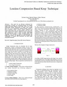
2. NLMS adaptive filters An adaptive filter has the property of self-modifying its frequency response to change the behavior in time, allowing the filter to adapt to the characteristics change of the input signal [11,12]. Due to this capability, the overall performance and the construction flexibility, the adaptive filters have been employed in many different applications like linear prediction. Adaptive filter encompass many different classic stochastic gradient algorithms [13].
Figure (1). Linear prediction layout using adaptive filter.
One common method is the Normalized Least Mean Square (NLMS) algorithm which is suitable for both stationary as well as non-stationary environment and provides a tradeoff between convergence speed and computational complexity [14]. In the case of an NLMS adaptive
http://technomag.bmstu.ru/en/doc/707364.html
355
FIR {
filter
tion
of
prediction order and the set of prediction coefficients = is a set of variables varying with time . The error of the predic-
of for each sample
is calculated by the expression: (3)
Where and
=
=
is the transpose operator.
The set of cooeffients
computed iteratively as follows: (4) (5)
(6) Where, - the convergence parameter, - the smoothing parameter (0 <