rna.vox. 7.97 great e ort is invested in reconstructing high-quality volumes. These are used for diagnosis, treatment planning, and scienti c observation for which ...
Lossless Compression of Volume Data James E. Fowlery Roni Yagelz yDepartment of Electrical Engineering
zDepartment of Computer and Information Science The Ohio State University Columbus, Ohio 43210
Abstract Data in volume form consumes an extraordinary amount of storage space. For e�cient storage and transmission of such data, compression algorithms are imperative. However, most volumetric datasets are used in biomedicine and other scienti c applications where lossy compression is unacceptable. We present a lossless data-compression algorithm which, being oriented speci cally for volume data, achieves greater compression performance than generic compression algorithms that are typically available on modern computer systems. Our algorithm is a combination of di�erential pulse-code modulation (DPCM) and Hu�man coding and results in compression of around 50% for a set of volume data les.
I. Introduction Compression for e�cient storage and transmission of digital data has become routine as the application of such data has grown. Several common datacompression programs are readily available on many computers to ght the burgeoning demand for storage space. These programs are typically generic; that is, they can compress data regardless of its nature. It is common that a single program is used to compress not only English text, but also source code, executable binaries, and raw data. Although generic programs have some advantages, such as greater portability, it may be worthwhile, in cases in which the demand for storage space is particularly high, to consider compression algorithms that have been tailored speci cally for a single application. One such application is volume graphics, the extension of computer graphics that addresses rendering directly from volume data. Since volume size grows as the cube of the resolution, even a moderateresolution volume requires a great amount of storage space. For example, consider a computer-tomography (CT) volume of 256 � 256 � 256 voxels. If each voxel has 16 bits of precision, a total of 32 Mbytes is needed to store this volume. It is easy to see that a collection
of several such volume images is unwieldy to maintain with today's technology. In this paper, we present a data-compression algorithm which, being oriented speci cally for volume data, will alleviate some of the storage-space problems associated with volume graphics. First, we present a very brief overview of general data-compression techniques. We then investigate previous attempts at volume compression. We follow this discussion with the details of our volume-compression algorithm. We conclude by comparing the performance of our algorithm on real volume data with that of several popular generic compression programs.
II. Data Compression Techniques Data compression is the encoding of a body of data, D, as a smaller body of data, D^ [1]. There are two general types of data compression: lossy and lossless. In lossless data compression, it is possible to reconstruct exactly the original data D given D^ . Such reconstruction is called decompression. Lossless compression is commonly used in applications, such as text compression, where the loss of even a single bit is unacceptable. On the other hand, in lossy compression, decompression produces only an approximation, ~ , to the original data D. Lossy compression is ofD ten used for applications such as image compression. Oftentimes with image compression, it is important that the decompressed image only looks like the original image; usually, it is not necessary to reproduce the image exactly, particularly if the image is being used for entertainment purposes. However, for applications such as medical imaging, lossy compression is unacceptable. Medical images are often used to identify tumors and other anomalies; distortion of the image due to compression may cause a false identi cation of a nonexistent tumor or the overlooking of a real one. In this paper, we will limit ourselves to the consideration of only lossless compression, as lossy methods are generally un t for data archiving. Moreover, volumes are used mainly in scienti c applications where
Lempel-Ziv (LZ) algorithm codes repeated variableTable 1: Voxel Entropies (in bits/voxel) of the Vol- length substrings as xed-length codes. LZ coding ume Dataset does not rely on prior knowledge of the source statistics but rather determines a \dictionary" of substrings Volume entropy from the source as coding progresses. For a well3dknee.vox 9.58 behaved source, the dictionary will contain strings CThead.vox 7.91 which have an almost equal probability of occurence. MRbrain.vox 7.93 Thus, dictionary strings containing frequently used 3dhead.vox 8.65 symbols are longer than those strings containing insod.30.vox 3.28 frequent symbols [6]. For a su�ciently well-behaved hipiph.vox 10.29 source, LZ coding achieves the lower bit-rate bound rna.vox 7.97 given by the source entropy of (1). These lossless compression techniques have been implemented in programs found on many UNIX sysgzip and zip (and PKZIP on MSDOS sysgreat e�ort is invested in reconstructing high-quality tems. tems) implement LZ compression as described above. volumes. These are used for diagnosis, treatment compress implements LZW compression [6], a variplanning, and scienti c observation for which lossy ant of the basic LZ algorithm. pack implements Hu�compression is unacceptable. Below, we discuss some man coding. Each of these programs designed to of the more common lossless techniques. Storer pro- compress computer les regardless of theis type of data vides a detailed discussion of these and other lossless- they contain. Below, we compare the performance of compression algorithms in [1]. each of these programs with our volume-compression algorithm on several volume data les.
III. Lossless Compression
IV. Volume Compression One of the most common lossless compression techniques is entropy coding, which capitalizes on the baDespite its extraordinary size, much of the inforsic tenant of information theory, entropy. Given a mation in a volume array is redundant. Although data source that outputs symbols from an alphabet, all data-compression techniques exploit data redun�, the entropy of the source is de ned as dancy to achieve compression, di�erent techniques do so di�erently. Lossless compression techniques such k X pi log2 pi (1) as Hu�man coding and LZ coding as discussed above H =? can be thought of as removing \statistical reduni=1 dancy" from the data. However, since we know that where k = j�j and pi is the probability of occurence our data is in the form of a volume, and that volumes of the ith symbol of �. It is assumed that the source possess some local spatial coherence, we can remove outputs the current symbol independently of the past this \spatial redundancy" as well to achieve greater outputs. Shannon's fundamental source-coding theo- compression. rem states that it is possible to code this source, withThere has been relatively little research reported out distortion, with an average of H + � bits/symbol, that deals directly with the issue of lossless volumetwhere � > 0 is an arbitrarily small quantity [2]. The ric compression. One early scheme was developed most common form of entropy encoding is Hu�man for the archiving of CT-image volumes and used runcoding [3], which attempts to match the source en- length encoding for very simple, yet very fast, lossless tropy by assigning shorter codes to source symbols compression [7]. Compression of 40% was typical for that occur frequently and longer codes to those sym- this scheme; however, a signi cant amount of this bols with small probability of occurence. Table 1 compression was due to the fact that 12-bit voxel inshows the entropy of the test volumes used later to tegers were stored with 16 bits each in the original generate results. These volumes are from the Chapel volume. Hill volume-rendering test dataset and are taken from There has been more interest in lossy volume comactual MRI, CT, and electron-density-map data. pression. Much of the early work in this area stemmed Another common technique of lossless compres- from attempts to compress television images by consion is the family of textural-substitution algorithms, sidering the sequence of frames as a volume. The use of which Lempel-Ziv [4, 5, 6] is the most popular. The of 3D transforms [8] is one approach that is equally
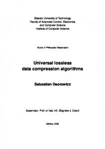
applicable to general volumes as it is to television + HUFFMAN data. An example of this approach is [9], in which a CODER Hadamard transform is used for real-time television − C compression. H PREDICTOR More recently, there has been some interest in A N lossy compression coupled with volume rendering [10, N 11, 12]. One proposal [10, 11] uses vector quantiE ENCODER L zation to compress the volume, resulting in greater speed of the rendering process. Since vector quantiza+ HUFFMAN tion is lossy, this algorithm is not suitable for archival DECODER + purposes. In [12], a discrete Hartley transform is used for compression. Again, this approach is lossy and PREDICTOR is intended to expedite the rendering process. Below, we present an algorithm designed speci cally for lossless compression of volume data that yields better DECODER compression than [7] and can be used for archiving. Additionally, it achieves greater compression than the Figure 1: Block diagram of the volumetric compresgeneric algorithms discussed in the previous section. sion algorithm d(x,y,z)
v(x,y,z)
~ v(x,y,z)
v(x,y,z)
d(x,y,z)
~ v(x,y,z)
V. Algorithm Details The algorithm we propose for volume compression is a combination of di�erential pulse-code modulation (DPCM) and Hu�man coding. Both techniques have been used extensively in compression of 2D images; for an overview, see [8]. Theoretical performance of entropy encoding to improve DPCM is discussed in [13]. DPCM belongs to a family of compression algorithms known as predictive techniques. In a volume, adjacent voxels usually possess a high degree of spatial coherence; that is, adjacent voxel values are highly correlated. Predictive techniques exploit this spatial coherence and encode only the new information between successive voxels. Predictive techniques feature a predictor that calculates a value from previously encoded voxels. This predicted value is subtracted from the current voxel. Thus, only the new information provided by the current voxel is encoded. Fig. 1 shows the block diagram of our volumecompression algorithm. The volume, v(x; y; z ), is read in raster-scan order. A predicted value, v~(x; y; z ), is subtracted from each voxel value, creating a stream of di�erence values, d(x; y; z ), which are then Hu�man coded. The channel shown in Fig. 1 is the archive system which is, in most cases, a disk drive. A. The Predictor The predictor is of the following form:
~(
)= ( ? 1; y; z ) + a2 v(x; y ? 1; z ) + a3 v(x; y; z ? 1)
v x; y; z
a1 v x
(2)
where v(x; y; z ) is the voxel array. Note that the predictor is causal; that is, the prediction is formed from only those values which have already been processed. Causality is required so that the decoder can track the operation of the encoder and generate the same predicted values as the encoder. The predictor coe�cients, ai , are determined so that the predictor is optimal in the mean-square-error sense. We must calculate new preditor coe�cients for each volume which we encode. The basic derivation of this calculation follows; more detail on optimal linear predictors can be found in [8]. To be optimal, the predictor must minimize the variance of the error sequence. The error sequence is (
� x; y; z
) = v(x; y; z ) ? v~(x; y; z )
(3)
and its variance is 2 �
= E [�2(x; y; z )]
(4)
where E [�] is the probabilistic expectation operator. This minimization occurs when the error is orthogonal to the voxels upon which we are basing the prediction: E [�(x; y; z )v(x ? 1; y; z )] = 0 (5) E [�(x; y; z )v(x; y ? 1; z )] = 0 (6) E [�(x; y; z )v(x; y; z ? 1)] = 0 (7)
"
After some algebra, we arrive at: (0 0 0) (1 ?1 0) (1 0 ?1) # " (?1 1 0) (0 0 0) (0 1 ?1) (?1 0 1) (0 ?1 1) (0 0 0)
r
r
;
r
;
;
;
;
r
;
r
;
;
r
;
;
;
;
r
;
;
a1
r
;
;
a2
r
;
;
a3
"
r r r
#
=
(1 0 0) (0 1 0) (0 0 1) ;
;
;
;
;
;
#
(8)
where r(x; y; z ) is the covariance of v(x; y; z ), (
r x; y; z
) = E [v(x0 ; y0; z 0 )v(x0 ? x; y0 ? y; z 0 ? z )] (9)
for Hu�man coding is presented in [8]. In our volumecompression algorithm, we use a variant of Hu�man coding called truncated Hu�man coding [8]. If the number of possible source symbols is L, the longest possible Hu�man code can have as many as L bits. Thus, in practical situations that require a large L, a truncated Hu�man code is used. In truncated Hu�man coding, the rst L1 symbols (L1 < L) are Hu�man coded and the remaining L ? L1 symbols are assigned a xed-length code. Thus, the maximum code length is restricted to a manageable length. For a volume with 16 bits per voxel, L = 131; 071 (16 bits/voxel implies di�erence values in the range ?66535 to 65536). For the lack of a suitable heuristic for choosing L1 , we arbitrarily set L1 = 256.
and x0, y0 , and z 0 are dummy variables over which the expectation is performed. Once we have determined the covariance, the predictor coe�cients, ai , are determined by solving the linear system of (8). In presenting this derivation, we make several as- C. The Compression Algorithm sumptions. First, we assume that v(x; y; z ) has zero mean. In general, real volume data will have a nonOur volume compression algorithm is given below. zero mean which we will have to subtract from To compress a given volume of size XY Z voxels, the v(x; y; z ) before we use (2). Secondly, we assume following steps are performed: that the volume is wide-sense stationary; that is, the 1. Scan the volume to estimate the mean: statistics (mean and covariance) do not vary through?1 YX ?1 ZX ?1 out the volume. For real volume data, this stationar1 XX v(x; y; z ) (10) v = ity does not hold { we will return to this point later. XY Z x =0 y =0 z =0 The predictor presented here is optimal in the mean-square-error sense. In many cases, this opti2. Scan the volume to estimate the covariance: mality may be overkill; good results may oftentimes be obtained from a simple predictor whose coe�cients ( )= are xed in advance. One such simple predictor is ob1 tained by setting a1 = a2 = a3 = 13 , which works rea( ? 2)( ? 2)( ? 2) � sonably well in practice if the voxel-sampling lattice ?2 �? ?2 ZX XX ?2 YX � is isotropic; i.e, the voxels are cubic. The advantage ( 0 0 0) ? � of the optimal predictor is that it will automatically x =1 y =1 z =1 �� ? compensate for non-isotropic sampling. In addition, (11) ( 0 + 0 + 0+ )? calculation of the optimal predictor is not very costly, for x; y; z 2 f?1; 0; 1g. as it takes only about 6% of the total compression time. 3. Calculate the predictor coe�cients, a1 , a2, and For simplicity, we have designed our predictor usa3, from (8) using the estimated covariance valing causal voxels from only the 6-neighborhood; i.e. ues. those voxels that share a face with the current voxel. 4. Scan the volume using the predictor to calculate Alternatively, one could include voxels from the 18the di�erence values, d(x; y; z ): or 26-neighborhoods (respectively, those voxels sharing an edge or a vertex with the current voxel). As d(x; y; z ) = v(x; y; z ) ? v ~(x; y; z ) (12) these voxels are more distant from the current voxel, v ~ ( x; y; z ) = a1 v1 (x; y; z ) + a2 v2(x; y; z ) + they will be less e�ective in prediction; however, fura3 v3 (x; y; z ) (13) ther study is warranted to determine whether the improvement they can o�er to the prediction is worth � the additional complexity of calculating more predic0 if x = 0 v ( x; y; z ) = 1 tor coe�cients. v(x ? 1; y; z ) ? v else (14) � B. The Hu�man Coder 0 if y =0 v2(x; y; z ) = An algorithm for the construction of a codebook v(x; y ? 1; z ) ? v else r x; y; z
X
Y
Z
v x ;y ;z
0
v x
0
v
0
x; y
y; z
z
v
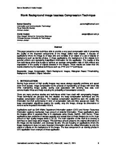
(15) Table 2: Exectution Times for the Compression Pro0 if z = 0 grams on 3dhead.vox. These times are for a HP 9000 v3 (x; y; z ) = v(x; y; z ? 1) ? v else Series 735. (16) Time (min) Method Compress Decompress 5. Count the number of times d(x; y; z ) = si for each possible si . These counts are the estimates compvox 4.7 1.4 of the symbol probabilities pi . compress 0.4 0.2 zip 0.8 0.5 6. Determine a truncated Hu�man code table usgzip 1.4 0.2 ing the pi probabilities. pack 0.2 0.3 7. Scan the volume once again, using the predictor to calculate the di�erence values, and the Hu�man code table to encode the di�erence values, compvox producing the compressed volume. gzip In the compressed volume, it is necessary to store compress the following, in addition to the coded di�erence val- 80% ues: 60% � The estimated mean, v. � The three predictor coe�cients, a1, a2 , and a3 . 40% � The Hu�man code table, which consists of the source symbols (di�erence values), si , and the 20% assigned Hu�man codes. One will notice that, in the course of compressing 3dknee CThead sod.30 hipiph a volume, the compression algorithm scans the volume four times. The rst two scans of the volume are used to estimate the mean and variance, respec- Figure 2: Percentage compression of several tively, of the voxels. Theoretically these two estima- data-compression programs on volume data tions could be done simultaneously in one scan; however, greater mathematical precision is obtained in 3. For each voxel in the reconstructed volume the estimate of the variance when the mean is already v(x; y; z ), calculate the predicted value v ~(x; y; z ) available. Since the mean and variance statistics are using (13). Read the next Hu�man code from needed only for the optimal predictor, if one chooses the compressed le and look up the di�erence to use the simple predictor as discussed previously, value, d(x; y; z ), in the Hu�man table for that these two scans for statistics calculation are unnecescode. Reconstruct the current voxel: sary. The last two scans of the volume are much more computationally intensive than the rst two. The last v(x; y; z ) = v ~(x; y; z ) + d(x; y; z ) (17) scan calculates the same di�erence values that were calculated during the third scan of the volume; however, to prevent excessive memory costs, these di�erences values are not saved, making a fourth scan of VI. Results the volume necessary. Table 2 compares the execution times for the different compression programs on one volume. Times D. The Decompression Algorithm for both compression and decompression are given. Table 3 compares the compression performance The decompression algorithm is as follows: of our volume compression algorithm, compvox, with 1. Read the estimated mean, v , and the predictor the compress , zip, gzip, and pack programs. Our coe�cients, a1 , a2, and a3 , from the compressed algorithm achieves the greatest compression for all le. the volumes except one. The volumes used here are 2. Read the Hu�man table from the compressed from the Chapel Hill volume-rendering test dataset le. and are taken from actual MRI, CT, and electron�
Table 3: Percentage Compression of Several Data-Compression Programs on Volume Data Volume
3dknee.vox CThead.vox MRbrain.vox 3dhead.vox sod.30.vox hipiph.vox rna.vox
Original Data
Resolution Size (Mb) 256 � 256 � 127 15.9 256 � 256 � 113 14.1 256 � 256 � 109 13.6 256 � 256 � 109 13.6 97 � 97 � 116 1.0 64 � 64 � 64 0.5 100 � 120 � 16 0.2 Average
compress
% Comp. 17.2% 46.0% 40.2% 29.9% 65.3% 26.8% 33.1% 36.9%
density-map data. Using compvox on the entire collection of these volumes saves 9 megabytes over compress. Fig. 2 is a bar graph of some of the data of Table 3 comparing the performance of compvox, gzip, and compress for all the volumes.
VII. Conclusions In this paper, we have presented an algorithm that is designed speci cally for the compression of volume data. From the results presented in Tables 2 and 3, one could conclude that, although our volumecompression algorithm yields compression superior to generic compression routines such as compress, zip, gzip, and pack, it requires signi cantly more processing time. However, the current implementation of compvox has not been optimized for execution speed; rather, it is prototype code that has been made exible to facilitate modi cations during the development of the algorithm. Greater attention to speed issues would make our code more competitive with the generic routines. As discussed previously, the optimal predictor that we design for each volume assumes that the statistics (mean and covariance) are wide-sense stationary throughout the volume. In any real volume, the best we can obtain is only some local stationarity; that is, the statistics are invariant only over small portions of the volume. One could obtain better predictions (and, thus, better compression) by designing a number of di�erent predictors, each optimized to a particular section of the volume, rather than choosing one predictor for the entire volume. We propose dividing the volume into an octtree, as is done in [14]. A separate predictor would be designed for each leaf node. A suitable criterion would determine the sizes of the leaf nodes based on the following tradeo�. With small leaf nodes, the predictors will be better able to ex-
zip
% Comp. 24.9% 48.9% 43.2% 33.8% 62.3% 28.5% 35.8% 39.6%
gzip
% Comp. 27.3% 50.3% 45.0% 36.1% 63.8% 33.2% 37.5% 41.9%
pack
% Comp. 27.3% 35.9% 37.2% 32.0% 58.4% 20.7% 35.3% 35.3%
compvox
% Comp. 40.1% 53.3% 52.7% 48.5% 63.7% 41.9% 55.4% 50.8%
ploit local stationarity. However, if the leaves are too small, not enough data would be available to precisely estimate the local voxel statistics. Somewhat similar approaches, wherein the predictor is changed as local statistics change, have been developed for 2D image compression; these approaches fall under the general heading of adaptive DPCM and are discussed in [8]. Localization of the predictor is one avenue we are currently pursuing to improve the compression performance of our algorithm. Additionally, we are examining whether increasing the neighborhood of the predictor from the 6-neighborhood to the 18- or 26neighborhood will appreciably improve performance, and a heuristic for determining the L1 value for the truncated Hu�man code is under exploration.
Acknowledgemets James E. Fowler is supported by a PhD Scholarship from AT&T. This research was supported by the National Science Foundation under grant CCR-9211288. We thank the University of North Carolina at Chapel Hill for the use of the volumetric datasets.
References [1] J. A. Storer, Data Compression: Methods and Theory. Principles of Computer Science Series, Rockville, Maryland: Computer Science Press, 1988. [2] C. E. Shannon, \A mathematical theory of communication," in Key Papers in The Development of Information Theory (D. Slepian, ed.), pp. 5{18, New York: IEEE Press, 1948. [3] D. A. Hu�man, \A Method for the Construction of Minimum-Redundancy Codes," Proceedings of the IRE, vol. 40, pp. 1082{1101, 1952.
[4] J. Ziv and A. Lempel, \Compression of Individual Sequences Via Variable-Rate Coding," IEEE Transactions on Information Theory, vol. 24, no. 5, pp. 530{536, 1978. [5] J. Ziv and A. Lempel, \A Universal Algorithm for Sequential Data Compression," IEEE Transactions on Information Theory, vol. 23, no. 3, pp. 337{343, 1977. [6] T. A. Welch, \A Technique for High-Performance Data Compression," Computer, vol. 17, pp. 8{19, June 1984. [7] M. L. Rhodes, J. F. Quinn, and B. Rosner, \Data Compression Techniques for CT Image Archiving," Journal of Computer Assisted Tomography, vol. 7, pp. 1124{1126, December 1983. [8] A. K. Jain, Fundamentals of Digital Image Processing. Englewood Cli�s, NJ: Prentice Hall, 1989. [9] S. C. Knauer, \Real-Time Video Compression Algorithm for Hadamard Transform Processing," IEEE Transactions on Electromagnetic Compatibility, vol. EMC-18, pp. 28{36, February 1976.
[10] P. Ning and L. Hesselink, \Fast Volume Rendering of Compressed Data," in Proceedings of IEEE Visualization, (San Jose), pp. 11{18, October 1993. [11] P. Ning and L. Hesselink, \Vector Quantization for Volume Rendering," in Proceedings of the Boston Workshop on Volume Visualization, pp. 69{74, ACM Press, October 1992. [12] C. Tzi-Cker, H. Taosong, A. Kaufman, and H. P ster, \Compression Domain Volume Rendering," 1994. Technical Report 94.01.04, SUNY at Stony Brook. [13] J. B. O'Neal, \Di�erential Pulse-Code Modulation with Entropy Coding," IEEE Transactions on Information Theory, vol. IT-22, pp. 169{174, March 1976. [14] D. Laur and P. Hanrahan, \Hierarchical Splatting: A Progressive Re nement Algorithm for Volume Rendering," Computer Graphics, vol. 25, pp. 285{288, July 1991.