Preprints of the 18th IFAC World Congress Milano (Italy) August 28 - September 2, 2011
LQG Control for Networked Control Systems with Random Packet Delays and Dropouts via Multiple Predictive-Input Control Packets Maryam Moayedi*, Yung K. Foo**, Yeng C. Soh*** *Nanyang TechnologicalUniversity, Singapore (Tel: 65-67906349; e-mail: mary0008@ e.ntu.edu.sg). **EW Electrical and Mechanical Engineering Private Limited, Singapore (e-mail:
[email protected]) *** Nanyang TechnologicalUniversity, Singapore (Tel: 65-67906349; e-mail: eycsoh @ ntu.edu.sg). Abstract: This article addresses the Linear Quadratic Gaussian (LQG) optimal control problem for networked control systems when data is transmitted through a TCP-like network and both measurement and control packets are subject to random transmission delays and packet dropouts. Instead of adopting a “zero-input” or “hold-input” strategy, we propose a “predictive optimal-input” strategy, where at each time instant, K future control inputs are computed and sent in addition to the current one in the same control packet. The stabilizability conditions of the system are then derived. Simulation results are presented to demonstrate the effectiveness of the proposed approach. class of NCSs under the effect of both delay and dropout where the full state vector is not available but assumed the network is only present between the sensor to the controller. [6] dealt with the control problem of networked systems in which random delays, packet loss and limitations of the communication channels between sensors, actuators, and controllers were taken into account. However, no stability analysis, taking the arrival probability of packets into account was presented. A Predictive controller where, at each sampling instant, a finite number ( K ) of future control inputs are computed and sent in addition to the current one in the same control packet (of size K +1) has been investigated in [8] via a “receding horizon” approach. It was then shown via simulations that under this scheme the overall performance of the closed-loop system, in terms of lower cost, has improved. However, the approach of [8] was developed to handle packet dropouts only (We acknowledge that this would not rule out applications of the approach to NCS involving both packet delays and losses because one could always discard a delayed packet and treat it as a lost packet). Moreover, the solutions obtained in [8] is dependent on the availability of some transitional probabilities, qij ’s ─ the
1. INTRODUCTION Networked control systems (NCSs) where data networks are used for connections between spatially distributed components of a control loop have recently attracted much attention. While using a communication network in NCS offers many advantages, it also leads to new challenges. Random time delay and data packet dropout are two main unavoidable problems in data transmission over unreliable communication networks,[10]. Usually the packets in NCSs suffer both random time-varying delays and dropout during the network transmission which would in general have a detrimental effect on the stability and performance of NCSs. Existing works in control and stability in NCS context mostly considered the packet loss or packet delay uncertainty in data transmission through the network. See for example [1]. However, we do remark that the results of [1] have been also extended to allow for a constant unit time delay in the control input, assuming the states are available to the controller for state feedback control. LQG optimal control problem over lossy TCP-like channels with randomly dropped sensor and control packets according to a Bernoulli process has been investigated in [12] and [11]. [3] also considered the problem of optimal LQG control when sensors and the controller are communicating across a packet erasure channel. There are quite a number of results considering both time delays and packet losses in NCSs. Most of them only considered the stabilization rather than performance e.g. [7], [17] or they assumed all of the states of the system are available for state feedback control, ([5]) or they considered delay and/or dropout in only one of the channels, [3]. In [4] and [7], discrete-time networked control system in the presence of random delays and dropouts is considered. However, both works assumed that all of the states are available to the controller for the state-feedback control. [17] addressed the stability analysis and synthesis problems for a Copyright by the International Federation of Automatic Control (IFAC)
probabilities of the system being in state j at time step k − 1 given that the system was in state i at time step k (i.e. a back-ward type of conditional probability, see equation 3 of [8]), and are hence quite tedious to compute. Apart from that, the complexity of the computations of qij ’s with increase in
K , increases exponentially. The problems with the availability of qij ’s and the corresponding computational complexity involving qij , as well as the desirability of considering both packet delays and dropouts in measurement and control packets with the stability analysis, motivate us to 72
Preprints of the 18th IFAC World Congress Milano (Italy) August 28 - September 2, 2011
propose a “predictive-input” strategy for the LQG control of networked control systems, with both measurement and control input packets subject to random delay and loss and where the states are not available to the controller. The paper is organized as follows. Section 2 will provide the mathematical formulation of the problem. In section 3, the optimal estimation problem with possible packet delay and dropout in both measurement and control input is studied. The controller design, i.e. predictive optimal inputs, is then derived in section 4. In section 5, the main results of the paper, i.e. the finite and infinite horizon LQG under TCP-like protocols via multiple predictive input control packets and the stabilizability analysis of the system with predictive optimalinput packets, are presented. In section 6, we give some examples to illustrate the applicability and effectiveness of proposed LQG filter-controller design schemes. Finally we give our conclusions in section 7.
However, because of network condition, the packet containing this information may or may not reach the actuator on time. As we have already mentioned, we assume the network adopted a TCP-like protocol, [11], so that the acknowledgement is always available to the controller, on time and with no loss, if the control packet has been received by the actuator. It has been shown that under such condition, the separation property holds and the optimal control law is in the form of u ( k ) = L ( k ) xs ( k / k ) where xs ( k / k ) is the Kalman estimate of x ( k ) (after measurement update, [11]) at time k . The objective of the estimation-control law is to minimize the following cost function: N −1
J N = E[ x ( N ) WN x ( N ) + ∑ ( x ( k ) Wk x ( k ) + u ( k ) U k u ( k )) | T
T
a
T
a
k =0
I N′ −1 , x0 , P0 ]
(2.2)
where I N′ −1 is defined in section 3, U k > 0 and Wk ≥ 0 . We
2. PROBLEM FORMULATION
k
define u ( k + i ) as the control input calculated by the controller at time step k corresponding to the optimal control input to be applied at time k + i . Thus the controller computes and dispatches a packet containing K + 1 projected
Consider the following discrete-time linear time-invariant system: a
x ( k + 1) = Ax ( k ) + Bu ( k ) + w( k ) z ( k ) = Cx ( k ) + v ( k )
k
k
k
control inputs {u ( k ), u ( k + 1), ..., u ( k + K } (instead of a packet containing only one control input u ( k ) ) at each
∑ α k ,i z ( k − i ); ∑ α k ,i = 1 if γ k = 1 y (k ) = i=0 (2.1) i =0 unavailable if γ k = 0 d
d
k
discrete time step k (Note u ( k ) is the same as u ( k ) ) from the estimation-control unit to the actuator. The actuator maintains a buffer to store one of the previous control packets received. If at time k a new control packet arrives, then it checks the time-stamp of this packet - if it is later than the one in the buffer, then it replaces the previous packet with this packet in the buffer. It then looks into the packet stored in the buffer and finds out how old it is. If this packet corresponds to a packet time-stamped (and hence dispatched by the controller) at time step k − m where m ≤ K , it then applies
a
where u ( k ) is the actual input applied to the actuator, y ( k ) is the measurement received by the estimator at time step k , { x (0), w( k ), v ( k )} are uncorrelated, white, with mean
{ x0 , 0, 0} and covariance {P0 , Q, R} , respectively, α k ,i are random variables that may take values of 0 or 1 only, which model the delay suffered by the measurement packets, d denotes the maximum delay a measurement packet is allowed (longer than which the packet would be discarded and treated as lost), and γ k is a Bernoulli random process with γ k taking
a
u (k ) = u {u
k −m
k−m
( k ) (Note that this packet would have contained
( k − m ), u
k −m
( k − m + 1), ..., u
k −m
( k − m + K } ).
Otherwise
a
value of either 0 or 1 with probabilities Pr(γ k = 1) = γ . The
(i.e. m > K ), it sets u ( k ) = 0 .
stochastic variable γ k models the loss of packets between the
We shall refer to this strategy as a “predictive-input” strategy. Obviously, to apply this strategy, we wish to
sensor and the estimator - if the estimator receives a measurement packet with a delay of no more than d steps at
k
k
k
compute {u ( k ), u ( k + 1), ..., u ( k + K } such that (1.2) is
discrete time k , then γ k = 1 , otherwise γ k = 0 .
k
minimized and it is required that u ( k + j ) will be in the
It is further assumed that arrival of packets from the controller to the actuator containing information about control input to be applied may be characterized by another sets of random variables β k , j that may take values of 0 or 1 to model
k
k
linear form of u ( k + j ) = Fk + j xs ( k + j ) where Fk + j are pre-
computable
off-line
and
xsk ( k +
j)
denotes the
best
(predictive) estimate of x ( k + j ) at time k . Note that this strategy requires the packet to contain K + 1 future control inputs, and this generally may be achieved without any additional communication cost, [8], if K is not excessively large.
the delay suffered by the control packets, and another {0,1}Bernoulli random variable ν k with probability Pr(ν k = 1) = ν to model packet losses. If the actuator receives a control packet with delay of less than or equal to some D at time step k , then ν k = 1 otherwise ν k = 0 .
3. ESTIMATOR DESIGN
Suppose the remote controller has decided that u ( k ) is the desired input to be applied at the actuator at time k .
3.1 Optimal State Estimation
73
Preprints of the 18th IFAC World Congress Milano (Italy) August 28 - September 2, 2011
The problem of the optimal state estimation under the conditions we have considered (i.e. with packet delays and dropouts) can easily be solved as in [9] or [10]. The reader is referred to the two references for more detail. We denote the
where β j = 1 if z ( j ) may be deemed available to the actuator at time step k , and β j = 0 otherwise. a
But because of the possibility of packet delays and dropouts between the controller and actuator, the computed desired control input u ( k ) = Fk xs ( k / k ) may not be available
k −m
k −m
k −m
k
k −1
ua
= {u
a
, u ak −1 } ,
y
k −m
known), then we may obtain
k −m
xsk ( k +
k −m
k
e
k −m
k −m
( k ) = x ( k ) − xs
k−m
Λ k ( k ) = E[ e
k−m
( k )e
(1 − ν )
(3.2)
k −m
(k )
T
| Ғk-m]
(3.3)
then
+ E[ e
0
j
j
T
j
k −m
k −m
T
(k ) S k e
k −m
j −1
k −m
( k )] = xs
T
( k ) xs ( k ) | I k′ ] = 0
(k )
T
k −m
( k ) S k xs
( k ) + tr ( S k Pk
k −m
N −1
T
T
k =0
+ν K ( k )u
k −m
T
(k ) U k u
k −m
( k ) | I N′ −1 , x0 , P0 ] (4.1) a
where ν K ( k ) = 1 if u ( k ) = u
k −m
( k ) where m may be any
value from 0 to K as explained before and ν K ( k ) = 0 if a
u ( k ) = 0 . To facilitate the computations of the control law, we approximate ν K ( k ) by an i.i.d. Bernoulli variable with probabilities
Prob{ν K = 1 }= (1 − (1 − ν ) K +1
K +1
)
and
.
Suppose that the best available estimate for x ( k ) deemed
(3.6)
k −m(k )
j
j −1
T
2
T
Pj = ( I − β j K j C ) Pj ( I − β j K j C ) + β j K j RK j
Pj j −1C T (CPj j −1C T + R ) −1 if β j = 1 Kj = if β j = 0 0
)
J N = E[ x ( N ) Ω N x ( N ) + ∑ E[ x ( k ) Wk x ( k )
function
Prob{ν K = 0 }= (1 − ν ) j −1
k −m
T
( k ) S k xs
k −m
time k . Therefore, we may consider the modified LQ cost
Update j to j + 1 k
T
( k ) | I k′ ] = E[e
Note that because the separation property holds, in general
(3.5)
xs ( k ) xs ( j ) = xs ( j ) + β j K j [ y ( j ) − Cxs ( j )]
( k ) = E[ x ( k ) | I k′ ] . Then the
the estimation x s ( k ) does not affect the controller gain at
(3.4)
Pj +1 = APj A + Q
.
Proof: Similar to lemma 4.1 of [11], with Ғk replaced by I k′ .
For j = k − d to k do (3.4)-(3.9): a
K +1
- E[ E[ g ( x ( k + 1)) | I k′ +1 ] | I k′ ] = E[ g ( x ( k + 1)) | I k′ ] , all g (.)
estimate of x ( k ) (deemed available to the actuator). The relevant equations for the optimal state estimates deemed available to the actuator at some future time k+j may then be (conceptually) computed as follows: Compute best current state estimate based on I k′ : j
k −m
( k )) xs
T
( k ) = E [ x ( k ) | I k′ ] = E [ x ( k ) | Ғk-m] would be the best
j
Suppose xs
- E[ x ( k ) S k x ( k ) | I k′ ] = xs
measurements which is “deemed available” to the actuator at time k . Clearly, if Ғk-m is the latest (and hence the largest set of) information (deemed) available to the actuator at time k , then we may denote the information deemed available to the actuator at time k by I k′ = Ғk-m. In such case,
xs ( j + 1) = Axs ( j ) + Bu ( j ), xs (0) = x0
k−m
k −m
Let I k′ denote the set of information on input and
xs
a
. Hence, the probability of u ( k ) = 0 is (1 − ν )
- E[( x ( k ) − xs
z ( j ) may be deemed available to the actuator at time step k .
k −m
(3.11)
following facts are true:
Correspondingly, y may be regarded as the set of measurements deemed available to the actuator at time step
k . Similarly if z ( j ) , j ≤ K − m is contained in y
K +1
Lemma 4.1:
k−m
k−m
T
The probability of K + 1 consecutive packet dropout is
(3.1)
(k )
k
(3.10)
4. CONTROLLER DESIGN (PREDICTIVE OPTIMAL INPUTS)
a
( k ) = E[ x ( k ) | Ғk-m]
k
j + 1) = [ A + BFk + j ] xs ( k + j ), j = 1, 2, 3, ..., K .
Pk + j+1 = APk + j A + Q
( k − 1), u ( k − 2), ..., u (0)} .
Define xs
k s
In particular, if u ( k + j ) = Fk + j x ( k + j ) (assuming Fk + j
= { y ( k − m ), y ( k − m − 1), ..., y (0)}, and
a
a
(3.9)
denotes the best estimate for x ( k ) based on the information set Ғk-m defined as follows: k −m
k
a
( k ) = Fk xs ( k ) at time k is xs ( k ) , where xs ( k )
Ғk-m ∆ { y
a
x s ( k + j + 1) = Ax s ( k + j ) + Bu ( k + j ); j = 1, 2, 3,..., K
to the actuator at time k . In fact, if m ( 0 < m ≤ K ) consecutive control packet dropouts have occurred immediately before time k , then the best state estimate that may be “deemed available to the actuator” (via
u
a
Furthermore, if u ( k ), u ( k + 1), ..., u ( k + K ) are known a priori, then the predictive state estimates may be given by the following recursive equation: Compute best future state estimates based on I k′ :
k
optimal state estimate at time k , as xs ( k ) .
available to the actuator at discrete instance k is xs
(3.7)
with the estimation error covariance Pk
k −m( k )
(k )
. We then apply
the dynamic programming approach based on the cost-to-go iterative procedure to derive the optimal control law. Define the optimal value function Vk ( x ( k )) as below:
(3.8)
74
Preprints of the 18th IFAC World Congress Milano (Italy) August 28 - September 2, 2011
T VN ( x ( N )) ∆ E[ x ( N ) WN x ( N ) | I N′ ]
j = 0,1, 2, ..., K . e. Controller dispatches control packet containing
(4.2)
T
Vk ( x ( k )) ∆ min E[ x ( k ) Wk x ( k )
k
+ν K ( k )u ( k ) U k u ( k ) + Vk +1 ( x ( k + 1)) | I k′ ] T
opt
theory, we know that J N = V0 ( x0 ) .
k −m
g. Actuator extracts u ( k ) from buffer and applies the control input to the system.
Lemma 4.2: For the system defined by (2.1) under TCP-like protocols, the value function Vk ( x ( k )) can be written as
Vk ( x ( k )) = E[ x ( k ) Γ k x ( k ) | I N′ ] + ck , k = N ,..., 0 T
5.2 Stabilizability of the System with Predictive Optimalinputs Packets For simplicity and ease of exposition we shall first consider the case of only possible packet dropout but not packet delay for the control packets, and later we extend it to possible delay and dropout in the control input. We know that delay in measurement in general does not cause the Kalman filter to diverge, [9]. Since the separation property applies for the TCP-like networked systems [11], for the purpose of analyzing the stability of the control scheme we shall assume γ = 1 and α k ,i = 0 for i ≠ 0 , for
(4.4)
where the matrix Γ k and the scalar ck may be computed recursively as follows: T
Γ
k +1
A
− (1 − (1 − ν )
K +1
T
−1
T
T
) A Γ k +1 B (U k + B Γ k +1 B ) B Γ k +1 A k −m(k )
T
ck = tr (( A Γ k +1 A + Wk − Γ k ) Em ( k ) [ Pk
(4.5)
])
+ tr (Γ k +1Q ) + E[ck +1 | I k′ ]
(4.6)
with initial values Γ N = WN and cN = 0 .
Moreover, the
simplicity. As mentioned earlier, at each discrete time k , we k
*
−1
k −m(k )
T
− (U k + B Γ k +1 B ) B Γ k +1 Axs −1
T
k −m(k )
( k ) = Fk xs
them in a control packet to the actuator. Thus, the optimal
( k ) (4.7)
T
where Fk ∆ − (U k + B Γ k +1 B ) B Γ k +1 A
input to be applied at time k is Fk xs ( k ) , where xs ( k ) is some
(4.8)
best minimum-error-variance estimate of x ( k ) available to the controller-actuator at time k . Restricting ourselves to the case where there is no delay (i.e. there is only packet dropout), we consider an equivalent system of which the controller is co-located with the actuator so that the controller-actuator knows what Fk is. Suppose the
Proof: Similar to proof of lemma 5.1 in [11], with Ғk replaced with I k′ , omitted due to space constraint. Remark 1: Note that in Lemma 4.2, we have expressed m as m ( k ) . This is because at different time k , the corresponding m may vary. We further note that the probabilistic distribution of m ( k ) in general depends on both γ and ν .♦
controller-actuator depends on “some” (fictitious) estimator (which is different from the real estimator of the closed-loop
5. THE MAIN RESULTS
system) to provide it with the best xs ( k ) and we assume any
5.1 Finite Horizon LQG under TCP-like Protocols via Multiple Predictive Input Control Packets Consider the system (2.1) and the problem of minimizing the cost function (2.2). Then the suboptimal control is a linear function of the estimated state given by equation (4.7) and (4.8) where the matrix is computed recursively by (4.5). The separation principle holds under TCP-like protocol. The optimal state estimator is given by (3.4)-(3.12). Therefore the combined estimation-control scheme may be summarized by the following conceptual algorithm: Conceptual Algorithm 1. Controller pre-computes Fk , k = 0,1, 2,..., N via (4.8).
xs ( k ) obtained and dispatched by the (fictitious) estimator
can reach the controller-actuator instantaneously and without a
k
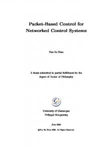
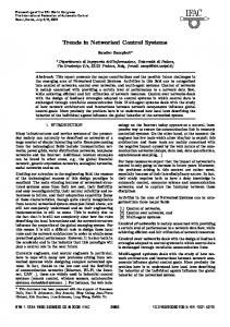
fail. Hence, the control input is u ( k + j ) = Fk + j xs ( k + j ) and the control action behaviour of the original system (with multi-control packet of size K and γ = 1 ) in Fig. 1 will be equivalently modelled by the control action behaviour of the equivalent system (with single-step-input control packet) shown in Fig. 2 with the following probabilities: Prob (control-packet loss between (fictitious) estimator and controller-actuator = 0; Prob (measurement loss between sensor and (fictitious) estimator = (1 − ν ) ;
At each k the following actions are performed: 2. Filter’s actions: a. Filter estimates xs ( k / k ) based on Ғk.
The (fictitious) estimator set xs ( k ) = 0 after it fails to receive
b. Filter dispatches xs ( k / k ) to Controller.
measurement in last consecutive K sampling time. It follows that the closed-loop system will be stable if and only if the “fictitious” state estimations are stable. Next, we consider the case in which delay is permitted. If delayed control packets are admitted, then when a delayed control packet arrives at the actuator at time step k , two cases could happen. The first one is when the packet has arrived
3. Controller’s actions: k
c. Controller assigns xs ( k ) = xs ( k / k ) and computes k
xs ( k + j + 1) , j = 0,1, 2, ..., K − 1 via (3.10) k
k
may set u ( k + j ) = Fk + j xs ( k + j ) , j = 0,1, 2, ..., K , and dispatch
optimal control decision is given by u ( k ) = T
k
4. Actuator’s action f. Actuator ensures control packet stored in buffer is the latest time-stamped packet received.
(4.3)
where k = N − 1, ...,1, 0 . Using the dynamic programming
Γ k = Wk + A
k
{u ( k ), u ( k + 1), ..., u ( k + K } to Actuator
u(k)
k
d. Controller computes u ( k + j ) = Fk + j xs ( k + j ) ,
75
Preprints of the 18th IFAC World Congress Milano (Italy) August 28 - September 2, 2011
before all of its successors. In such case, it will be stored in the buffer for control purposes (and hence considered “useful”) and we may deem it as a delayed measurement has arrived. However, if it arrives after one or more of its successors, it will be discarded and treated as a lost packet. Nevertheless, all the measurements that are deemed to have incorporated, would have been incorporated by its successors arrived earlier, so no information is actually lost despite its being discarded. Hence, a delayed control packet arrival may be deemed as a delayed measurement arrival at the actuator. Since delays in measurements in general do not lead the state estimations to instability as long as they arrive eventually [9], employing the same argument as above shows the stability of the overall closed-loop will not be affected by the delays of the control packets, if γ = 1 . Actuator
Plant
1/ 2
( A, Q ) , ( A, B ) be controllable and R > 0 . Suppose A is diagonalizable and the unstable eigenvalues of A are distinct. Assume the probability of measurement packet loss between the sensor and the estimator is 1 − γ and the probability of the control packet loss between the controller and actuator with control packet of size K + 1 is 1 − ν . Then the system can be stabilized via a linear regulator using multiple predictive optimal-input control packets of size K + 1 and zero-input strategy if −1
(5.2)
i
u
where λi ( A) are the unstable eigenvalues of A .
Proof: The proof is omitted due to space constraint. Remark 2: Proposition 5.2 implies theorem 5.1 holds. ♦
Sensor
5.3 Infinite Horizon LQG under TCP-like Protocols via Multiple Predictive Input Control Packets Theorem 5.1 (Infinite Horizon LQG under TCP-like protocols via multiple predictive input control packets): If Wk = W and U k = U are constants, then a positive definite
Network
solution for Γ ∞ exists for the following discrete-time Riccati
Estimator-Controller Measurement loss probability: 0, i.e. γ =1
Control packet loss probability : 1 − ν
2
u
γν > 1 − (max | λi ( A) | )
equation Γ ∞ = T
W + A Γ ∞ A − (1 − (1 − ν )
Figure 1. Original system with multi-control packet of size K+1
(1 − (1 − ν )
K +1
K +1
T
−1
T
T
) A Γ ∞ B (U k + B Γ ∞ B ) B Γ ∞ A. if u
2
−1
) > 1 − (max | λi ( A) | ) . Furthermore, the i
k
Controller-Actuator
Plant
k
multiple-input control packets with u ( k + j ) = F∞ xs ( k + j ) ,
Sensor
j = 0,1, 2, ..., K , stabilizes the system in closed-loop with F∞ ∆ T
−1
T
u
2
− (U + B Γ ∞ B ) B Γ ∞ A if γν > 1 − (max | λi ( A) | )
Network
−1
i
u
where λi ( A) are the unstable eigenvalues of A . Estimator
Proof: The proof is omitted due to space constraint. Measurement loss probability: 1 − ν
State estimate loss Probability: 0
6. EXAMPLES
Example 1: We consider the system used in [8]: 1 1 0 A= , B = 1 , C = [1 0 ] 0 1 The noise processes v ( k ) and w( k ) are assumed to be zero
Figure 2. Equivalent system with single-step control packet.
We may now state our results on stabilizability. The following propositions are used to establish necessity condition and sufficient condition for stabilizability: Proposition 5.1 (necessary condition): Suppose A of
mean, with variances R = 0.5 and Q = I 2×2 respectively.
1/ 2
T
) and ( A, B ) be controllable and R > 0 . Assume the probability of control packet loss between the controller and actuator is 1 − ν . Then the system cannot be stabilized via a linear regulator using multi-predictive optimal input control packets with finite K and zero-input strategy if u
2
ν ≤ 1 − (max | λi ( A ) | )
−1
T
N = 30 (horizon length), Wk = C C , U k = 0.3 , WN = C C
system (2.1) is unstable. Let ( A, C ) be observable, ( A, Q
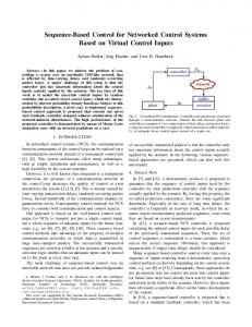
(final cost-weight matrix) and x (0) = 0 . We use the same estimation scheme and compare the performance of the timevarying predictive optimal input controller with control packet size K + 1 where K = 0,1, 2, 3 and 4. We construct and simulate results using γ = 1 and ν = 0.6, 0.7, and 0.8. The average (over 200 simulations) of empirical costs versus different values of control packet arrival probability is shown in Fig. 3 where we have incorporated the performance of the single-control packet based zero-input strategy and hold-input strategy for comparison. We note that K = 0 is equivalent to zero-input strategy of [11].
(5.1)
i
u
where λi ( A) are the unstable eigenvalues of A .
Proof: The proof is omitted due to space constraint. Proposition 5.2 (sufficient condition): Suppose A of system (2.1) is unstable. Let ( A, C ) be observable,
76
Preprints of the 18th IFAC World Congress Milano (Italy) August 28 - September 2, 2011
Table 1. LQG cost for predictive-input controller with different values of K for the two cases: (1) all delayed control packets are treated as packet dropout case ( ν = 0.6 ); (2) any control packet with delay of more than one-step is treated as packet dropout ( ν = 0.72 ).
1.5 LQG cost
1.3 K=0 (Zero-input) K=1 K=2 K=3 K=4 Hold-input
1.1 0.9 0.7 0.5
J K =0
J K =3
J K =4
1.6708 1.3075 1.1661 1.1232 1.1084 1.4951 1.1843 1.1195 1.1046 1.1007 From the table, it is clear that when ν = 0.72 , the LQG cost for predictive-input controller would be smaller than the cost for the case ν = 0.6 for different values of K . In other words admitting a one-step delayed packet as a delayed packet (i.e. not a lost one) in the controller design, helps to improve the system performance.
0.1 0.7 ν
J K =2
ν = 0.6 ν = 0.72
0.3 0.6
J K =1
0.8
Figure 3. LQG cost for different controllers versus control packet arrival probability 0.45
ν=0.6 ν=0.7 ν=0.8
LQG Cost
0.4
6. CONCLUSIONS
0.35
In this paper, we considered the LQG control problem over a communication network where both the measurement and control may be delayed or lost. We adopted a multiple-control packet-based predictive-input strategy. Simulations results showed that the strategy proposed in this paper performs better than the single-control packet based zero-input strategy and the hold-input strategy.
0.3 0.25 0.2 0
1
2
3
4
K
REFERENCES
Figure 4. LQG cost vs. number of control inputs per packet for different probabilities of control packet arrival.
[1]
Wang, Z., F. Yang, D. W. C. Ho and X. Liu (2007). Robust
H∞
control for networked systems with random packet losses. IEEE Trans. Systems, man and cybernetics, 37, 916-924. [2] Moayedi, M., Y.K. Foo and Y.C. Soh (2010). Optimal and suboptimal minimum-variance filtering in networked systems with mixed uncertainties of random sensor delays, packet dropouts and missing measurements. Int J. Cont. Autom. and systems. 58, 1577-1588. [3] Gupta, V., B. Hassibi, and R.M. Murray (2007). Optimal LQG control across packet-dropping links. Systems and Control letters, 56, 439-446. [4] Li, H., M.Y. Chow and Z. Sun (2009). Optimal stabilizing gain selection for networked control systems with time delays and packet losses. IEEE Trans. Contr. System Tech., 17, 1154-1162. [5] Li, H., Z. Sun , M.Y. Chow, and B. Chen (2008). State feedback controller design of networked control systems with time delay and packet dropout. In proceedings of the 17th IFAC Congress, 6626-6631. [6] Matveev, A.S., A.V. Savkin (2004). Optimal control via asynchronous communication channels. Journal of Optimization Theory and Applications, 122, 539-572. [7] Rivera, M.G., A. Barreiro (2007). Analysis of networked control systems with drops and variable delays. Automatica, 43, 2054-2059. [8] Gupta, V., B. Sinopoli, S. Adlakha, A. Goldsmith and R. Murray (2006). Receding Horizon Networked Control. Proceedings of 44th Annual Allerton Conference, 169-176. [9] Schenato, L. (2008). Optimal estimation in Networked Control Systems subject to random delay and packet drop. IEEE Trans. automat. Contr., 53, 1311-1317. [10] Moayedi, M., Y.K. Foo and Y.C. Soh (2010). Filtering for Networked Control Systems with single/multiple measurement packets subject to multiple-step measurements delays and multiple packet dropouts. Int J. Syst Science. 42, 335-348. [11] Schenato, L., B. Sinopoli, M. Franceshetti, K. Poolla, and S.S. Sanstry (2007). Foundations of control and estimation over lossy networks. Proc. of IEEE, 95, 163-187. [12] Imer, O.C., S. Yuksel, and T. Basar (2006). Optimal control of dynamical systems over unreliable communication links. Automatica, 42, 1429–1440.
Fig 4 plots the LQG costs versus different number of control inputs per packet for different probabilities of control packet arrival. From Fig 4, it can be seen that the LQG cost decreases as the number of control inputs per packet is increased but it is getting flatter as the number of control inputs is further increased, especially for higher probabilities of control input arrival. This is because for high probabilities of arrival, the chance of consecutive packet dropouts is small One may take the “knee-point” of leaving-off as the “optimal” packet size. Next, we focus on ν = 0.6 to investigate the effect of admitting a one-step delay. Let ρ1 , ρ 2 and ρ3 denote the probabilities that the packet which arrives at the actuator is a current control packet, a one-step delayed control packet, and one with more than one-step delay or no packet arrives at the actuator respectively. We assume that by admitting a one-step delay, the value of ν may be increased to 0.72 (with ρ1 = 0.6 , ρ 2 = 0.12 and ρ3 = 0.28 . Note that ρ1 and ρ 2 are not required for the purpose of controller design and if we decide not to admit the one-step delay control packet and discard it and treat it as a packet loss, then ν decreases back to 0.6.) The average of the empirical costs over 200 simulations versus K = 0,1, 2, 3 and 4 have been computed and tabulated in table 1 below. For a more realistic simulation with precedence constraint [2], we have used the following conditional probabilities for the simulation of one-step delays and packet dropouts ( ρi / j = Pr (the system is at state i at time step k | the system has been at state j at time step k − 1 , [2]) : ρ1/1 = 0.6 , ρ1/ 2 = 0.6 , ρ1/ 3 = 0.6 , ρ 2 /1 = 0
ρ 2 / 2 = 0.3 , ρ 2 / 3 = 0.3 , ρ3/1 = 0.4 , ρ3/ 2 = 0.1 , ρ3/ 3 = 0.1 . 77