LSB neural network based segmentation of MR brain images Yan Li*,
Peng Wen* , David Powers* and C. Richard Clark**
*Artificial Intelligence Laboratory School of Informatics and Engineering The Flinders University of South Australia GPO Box 2100, Adelaide, SA 5001, Australia. {yan.li, peng.wen, david.powers}@flinders.edu.au **Cognitive Neuroscience Laboratory School of Psychology The Flinders University of South Australia
[email protected] ABSTRACT Least Square Backpropagation(LSB) algorithm is employed to train a three-layer neural network for segmentation of Magnetic Resonance(MR) brain images. The simulation results demonstrate the use of LSB neural Network as a promising method for the segmentation of multi-modal medical images. The training time has been dramatically reduced comparing with that of BP network. The influence of the number of neurones in the hidden layer of the network is discussed in the paper.
1. INTRODUCTION Neural networks have over the last decade been successfully applied to many image processing tasks[1,2]. Their major advantage is that they don’t depend on any assumption about the underlying probability density functions, thus possibly improving the results when the data significantly depart from normality. One particular application area where neural networks show some promise is the field of Magnetic Resonance (MR) image segmentation. Most previous studies of neural network based MR image segmentation have employed the backpropagation (BP) algorithm. M. Ozkan and B. M. Dawant[3, 4] presented a BP neural network approach to the automatic characterisation of brain tissues from multimodal MR images. In their papers, the ability of a threelayer BP neural network to perform segmentation based on a set of images acquired from a pathological human subject were studied. The results were compared with those obtained using a traditional Maximum Likelihood Classifier(MLC). Neural networks-based segmented images appear less noisy than MLC segmented images,
and it has been observed that the Neural Networks Classifier(NNC) is also less sensitive to the selection of the training sets than the MLC. In spite of the fact that confusion matrices do not indicate significant difference between NNC and MLC. The BP algorithm, however, has a very slow convergence rate and requires a priori learning parameters. These drawbacks have significantly limited the application of neural networks in this area, especially since the MR images training sets required are very large. Recently, several improved training algorithms have been reported in the literature. One of these methods, the Least Square Backpropagation (LSB), operates by looking at the structure of neural networks, separates the neural networks into linear and non-linear parts, and then optimises the linear part of each layer from the output layer to the input layer using the least square method. The main advantage of the LSB algorithm is that it can converge within less than 10 iterations. It therefore makes possible the application of neural networks for medical image processing where large training sets are required. MR imaging is unique among diagnostic imaging modalities because it employs several independent parameters which determine the image scale. The image intensity permits the detailed visualisation of the internal anatomical structures in living human subjects. MR image parameters include tissue relaxation times: the spin-lattice relaxation time (T1) and the spin-spin relaxation time (T2), and the proton density (PD). The goal of MR image segmentation is to accurately identify the principal tissue structures in these image volumes. Least square backpropagation algorithm is employed to train a three-layer neural network for segmentation of
MR brain images in this paper. The methodology is briefly described in the next section. Some segmentation results are given in Section 3. Finally, section 4 contains the conclusion of this paper.
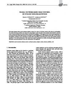
2. METHODOLOGY 2.1 LSB algorithm A learning algorithm for multilayered neural networks based on linear least squares problems, was presented by Friedrich Biegler-Konig and Frank Barmann[5] in 1993. Konig and Barmann separated neural networks into linear parts, summations of the weighted inputs to neurones and non-linear parts, non-linear activity functions (such as sigmoidal activation). While solving the linear parts optimally, they used the inverse of the activation to propagate the remaining error back to the previous layer of the neural networks. Therefore, the learning error is minimised on each layer separately from the output layer to the hidden and input layer by using least square method. Before proceeding to derive briefly the training algorithm, it is necessary to give an explicit description of a three-layer feedforward neural network. The architecture of such a network is shown in Fig.1, where I and O are the input and output of the network, respectively. The network may be represented in block diagram form as a series of affine transformations W1 and W2, and a diagonal non-linear operator f with identical sigmoidal activations. In other words, each layer of the network is regarded as the composition of an affine transformation
As it is observed, a three-layer neural network is denoted by S(W1,W2), here W1 and W2 are the weights of the connection. A is the output of the hidden layer in the network. Propagating the given examples through the network, we get (by multiplying the input matrix with the weights matrix between input layer and hidden layer, applying the activation function to all matrix elements, and adding a bias constant column of 0.5).
A = [ 0 .5 | f ( I * W 1 ) ]
(3)
O = f ( A *W 2)
(4)
where A and O are the outputs of the hidden layer and output layer. Teaching the network means trying to adjust the weights such that O is equal to (or as close as possible to) D, here D is the desired output of the network. By introducing R = f- - 1(D)
(5)
Let us reformulate the task of learning: Adjust the weights of the network such that R is as close as possible to A*W2. The problem of determining W2 optimally can be formulated as a linear least squares problem: minimize||A*W2-R||2
(6)
Note that, since f is a non-linear function, the minimum of equation (6) is not necessarily identical with the minimum of || O -D ||2.
A W1
After obtaining an optimal set W2 of weights, we could determine a required output matrix Da of hidden layer which is as close as possible to A and fulfils
W2
I
O
• •
• •
• •
• •
• •
One iteration is finished by updating the weights W1 , W2. 2.2 MR brain images segmentation using neural networks
with a non-linear mapping:
O = f( A*W2 )
(7)
Again, this is for given matrix W2 and R, a linear least square problem. After Da obtained using Equation (7) , W1 can be solved as above using Equation (5) & (6).
Figure 1 The architecture of a three-layer neural network
A = f( I*W1 )
minimize|| Da*W2 - R ||2
(1) (2)
The above three-layer neural network is employed to analyse MR images in this paper. The inputs to the network are the corresponding T1-weighted, T2weighted, and PD image intensity values for each pixel. The resulting six outputs of the network are the
segmented tissue classes, namely the scalp, skull, CSF, cortex(graymatter), white matter, and background. Their values range from 0 to 1, indicating the degree of membership of the tissue within the certain tissue class. The training samples are a set of pixel-type pairs that are arbitrarily taken from pre-segmented images. Additional experiments were performed with the pixel’s coordinates as extra inputs to the neural network. The results were defected for the additional complexity and training time, but no visible improvement in the segmented images.
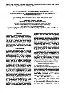
3. SIMULATION RESULTS. PD modality Figure 2 The planar pre-segmented T1-weighted, T2-weighted and PD images Some segmentation results about the proposed approach are presented in this section. MATLAB is used to implement these simulations in Sun workstation. The performances of LSB-based segmentation are compared with those of traditional BP algorithm.
T1-weighted
T2-weigted
The pre-segmented MR images used in this paper are obtained from the http://www.bic.mni.mcgill.ca/brainweb web site. The brain phantom and simulated MR images have been made publicly available and can be used as gold standard to test analysis algorithms such as classification procedures which seek to identify the tissue ‘type” of each image voxel[6]. The three modalities, T1-weighted, T2weighted and PD are downloaded as pre-segmented images. The training sets are selected from the representative regions of interests. The anatomical models provided in the above web site can be used as the standard information for choice of region of interest for the segmented tissue types. To guarantee the correct sampling on all the modalities and anatomical models, the training set are selected arbitrarily according to the coordinates on one of the images and are automatically echoed on all others. The pixel’s coordinates, intensity values, and class memberships are then stored on file as a training set. For testing set, another set of data are arbitrarily selected in the same way. Figure 2 shows the planar pre-segmented T1-weighted, T2-weighted and PD images used in the study. The simulation results show that the training process can converge within 4 iterations using the LSB algorithm, even though there are large number of training samples. Some segmented tissue types, graymatter and scalp are shown in figure 3 when the number of neurones in the hidden layer is 12. There are 5000 training samples in this case. It takes 31.75 seconds(including sampling the
training data from the pre-segmented images) for the LSB method, while a conventional BP network needs 71743 seconds, almost 20 hours, to achieve a comparable performance shown in figure 3. From figure 3, it is observed that there is little ‘pepper and salt’ in the images.
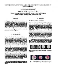
Above 48 nodes in the hidden layer of the network, no significant improvement could be observed though the training error still decreases a little. Similar results apply to other tissues, Skull, CSF and White matter.
The performance continues to improve as the number of the neurones in the hidden layer increases. Figure 4 shows the segmented images when the number of the neurones in the hidden layer is 48. The training error, mean sum squared error(SSE), can be as small as 0.0586 for 5000 training samples once the training process is completed in this case. The minimum test error for the same number of samples taken arbitrarily from the images is 0.0639. There is no difference between the segmented images and the anatomical models from the visual point of view. It takes 49.26 seconds for LSB algorithm, more than 53 hours for BP to achieve comparable results( SSE