Machine Learning for Subproblem Selection
Robert Moll
[email protected] Theodore J. Perkins
[email protected] Andrew G. Barto
[email protected] Department of Computer Science, University of Massachusetts, Amherst, MA 01003
Abstract Subproblem generation, solution, and recombination is a standard approach to combinatorial optimization problems. In many settings identifying suitable subproblems is itself a significant component of the technique. Such subproblems are often identified using a heuristic rule. Here we show how to use machine learning to make this identification. In particular we use a learned objective function to direct search in an appropriate space of subproblem decompositions. We demonstrate the efficacy of our technique for problem decomposition on a particular wellknown combinatorial optimization problem, graph coloring for geometric graphs.
1. Introduction Subproblem generation, solution, and recombination is a standard technique in combinatorial optimization. Often this “divide and conquer” method involves a search for one or several suitable subproblems, and the outcome of this search can critically affect the performance of the overall algorithm. For example, in a classical vehicle routing problem in Operations Research, a fleet of vans, each with a fixed carrying capacity and each starting from a common depot, is given the job of making deliveries to a set of sites and then returning to the depot. The deliveries assigned to any van must not exceed that van’s carrying capacity. The problem objective is to assign deliveries to vans, and then route each van so as to minimize the total travel distance of all of the vans. Clearly, how sites are assigned to vans, that is, which subproblems are generated, is critical for obtaining a good overall problem solution. Classroom scheduling presents a more mundane example of this phenomenon. Suppose a school administrator is presented with a computer-generated classroom schedule that makes poor use of a popular
classroom. The administrator might then generate a subproblem — improve the usage of this room — and will often solve the subproblem manually by shifting room assignments until a more suitable arrangement is found. How subproblems are identified, e.g., which sites are assigned to which vans, or which classrooms should be targeted for improved scheduling, is often done heuristically. Here we describe an alternative approach to subproblem selection. Our method first identifies an abstract space of subproblems, and then uses machine learning to make search feasible in this space. While in principle we do not restrict the form of this search, in the example presented here we use local search over a suitably formulated space of subproblems. Suppose an optimization problem, such as the vehicle routing problem described above, can be solved by first decomposing it into subproblems from some class C, and then by solving those subproblems. In the vehicle routing example, class C consists of collections of single van routing problems. Our technique involves searching C for a particularly promising member of the class, and then solving the resulting subproblem(s). Searching C involves the use of some algorithm, A, which solves instances from C (e.g., A might be an algorithm for routing a single vehicle efficiently). Since using algorithm A explicitly for this search is frequently too expensive, the feasibility of the search depends on being able to estimate algorithm A’s performance quickly on example subproblems. To accomplish this we first identify a set of quickly computable features that can be used to capture, with some precision, the expected behavior of A on any instance. Then, using supervised learning in an off-line training ˜ procedure, we create A(·), an estimate of A’s performance. This is done by running A on a large corpus of examples, and then using regression to adjust function approximation parameters to fit A’s output values. Once constructed, we use A˜ — a fast, inex-
pensive substitute for A itself — as a cost function for hillclimbing in subproblem space C. When we arrive at a local optimum in this space, we apply A to the subproblem or subproblems associated with the optimum, and use the results obtained to form an overall problem solution.
ing, register allocation for compilers, and VLSI layout. We illustrate our subproblem selection technique by examining the graph coloring problem for a particular subclass of graphs, namely geometric graphs. These graphs model the channel assignment problem for mobile communications systems.
A number of investigators have studied the use of a learned cost function to direct local search. Zhang and Dietterich (1995) consider instances of a NASA space shuttle mission scheduling problem. Using reinforcement learning (Sutton & Barto, 1999), they develop a local search-like technique for removing constraint violations from infeasible schedules. Boyan and Moore (1998) develop a technique for acquiring a hillclimbing cost function on-line. They simultaneously learn this function and use it to search for good initial solutions from which to begin conventional local search. Their STAGE algorithm works on specific instances of deterministic optimization problems. Our work (Moll, et al., 1999) shows how to use a learned value function directly as a generalized cost function within the framework of conventional local search. That work is concerned with demonstrating a methodology for acquiring and then using a learned cost function for standard local search across all instances of a problem class.
A coloring of an undirected graph is an assignment of colors (e.g., distinct integers) to vertices, with the property that adjacent vertices (vertices connected by an edge) have different colors. Thus a coloring partitions vertices into classes, such that members of the same partition or color class are not adjacent. An optimal graph coloring partitions the vertices of a graph into the fewest possible color classes.
All three studies cited above investigate the efficacy of learning a cost function for searching spaces of feasible (or, in the case of Zhang and Dietterich, infeasible) solutions. The approach in this paper operates at a different level. We employ local search over a space of viable subproblems in a generalized divide and conquer setting in an attempt to find subproblems that are most promising with respect to the estimated behavior of a known algorithm. We illustrate our technique by examining its effectiveness for improving graph coloring for a class of geometric graphs. In (Moll, Perkins, & Barto, 1999) we discuss this problem, as well as the application of our technique to a problem we call the Multiple Uninhabited Air Vehicle Surveillance Problem, or MUAV, a stochastic, traveling salesman-like problem. We describe our work on the MUAV problem briefly in Section 3.
2. Graph Coloring Graph coloring is one of the most widely studied NPcomplete combinatorial optimization problems, and has many important applications, including schedul-
For the class of random geometric graphs we consider, vertices correspond to uniformly randomly generated points in the unit square. Two vertices are adjacent in the graph if the distance between their corresponding points falls below a certain threshold. UN,t denotes the class of random geometric graphs on N points with adjacency determined by distance threshold t. A widely studied threshold, and the one we consider in this paper, is t =.5. In the case of graph coloring for geometric graphs we proceed as follows. Let C be a subclass of geometric graphs, determined, for example, by parameter t, and let A be any coloring algorithm. We first construct ˜ which can quickly estimate the estimator function A, behavior of A on a graph in C, i.e., the number of colors A uses to color that graph. (We describe this construction shortly). Once A˜ has been constructed, we use it to augment our original algorithm A as follows. Let G be an arbitrary geometric graph. First we color G using A. Then we identify a set of color classes where we believe the coloring has been inefficient. Here we choose small classes, because it is more likely that by combining their members and then recoloring, we will be able to reduce the number of colors required. Thus recoloring the members of these small classes becomes the subproblem we wish to attack. However there may be other subproblems, obtained by exchanging vertices in this set with other still-colored vertices, that could be more promising for recoloring using A. The essence of our method is to use A˜ as a hill-climbing cost function to search through these subproblems until we arrive at a (locally) most promising one. Then we color that collection of vertices vertices using A. More specifically, our method, applied to (geometric) graph coloring, can be described as follows.
Given geometric graph G, first color G using A. Then: 1. Select a subset of color classes that are appropriate for reorganization into fewer classes (e.g., some of the sparsely populated color classes). Collect the vertices in these classes into a “recolor” set. The collection of vertex sets that are the same size as this set constitutes the space of subproblems to be considered. 2. Using standard first-improvement local search flow of control (Papadimitriou & Steiglitz, 1982), hill climb in the space of recolor sets by repeatedly considering pairwise exchanges between vertices in the current recolor set and vertices in some still-intact color class S. A swap is accepted if it preserves the integrity of S (here: the alteration of S should introduce no adjacencies to S, i.e., no vertices in S should be linked by an edge), and if ˜ estimate of A’s performance on the recolor set A’s is improved by the exchange. 3. When a local optimum is reached in 2), solve the subproblem by applying A to the newly constituted recolor set. 4. Once this subproblem has been solved, combine its coloring scheme with the other color classes (which may be slightly altered as a result of the exchange process, but which are still legal classes) to get a complete, optimized solution to the problem. 2.1 Graph Coloring Results We considered geometric graphs from the classes UN,t with 250, 500, and 750 vertices, and for distance threshold t = .5. At these three sizes, graphs in UN,.5 have roughly 14,000, 60,000, and 130,000 edges respectively. For our base algorithm A we use the DSATUR algorithm (Brelaz, 1979). This algorithm is reported to be the best, or at least competitive with the best algorithms known for geometric graphs (Johnson et al., 1991). It works as follows: Let G be an undirected graph, Form a random permutation of G’s vertices. While vertices remain uncolored: 1. Choose the uncolored vertex adjacent to the highest number of distinct colors among the already colored vertices. (Break ties by taking the lowestindexed vertex.)
2. Assign the lowest-indexed legal color to that vertex. Notice that since vertices are presented in random order, any ties in 1) are also broken randomly. For our estimation function A˜ for DSATUR we use a linear function approximator. It is constructed using regression from normalized versions of two features and their squares. These features are: the number of edges in the graph (E), and the variance of the degrees of the vertices (V). Our function approximator is: g DSATUR(E, V)= (−1.78 ∗ E) + (2.18 ∗ E 2 ) + (−.36 ∗ V ) + (.47 ∗ V 2 ) + .77 Feature normalization is necessary to account for the size variation across problem instances in the class of recolor vertex sets that are to be searched. Suppose that Vraw represents the unnormalized variance of a particular instance. Then we divide Vraw by a quadratic polynomial in the problem size, N , to determine the normalized variance, V. We also used regression to determine the coefficients of this polynomial: we constructed several thousand example geometric graphs of various sizes, and then did a least-squares fit to determine values for α, β, and γ such that Vraw satisfies Vraw /(α + β ∗ N + γ ∗ N 2 ) = .5 The result of this regression then yielded the coefficients α, β, and γ, for the sought-after normalizing polynomial. g We constructed DSATUR by applying linear regression to DSATUR’s performance on 10,000 example geometric graphs from sizes 10 to 80 (the approximate size range of recolor vertex sets). For each example graph G we calculated the normalized feature values E, E 2 , V , and V 2 . We also calculated a target value, the result of applying DSATUR to the graph in question (number of colors used), divided by the number of vertices in the graph. We then used linear regression g to fit DSATUR’s weights to these target values. The size of the recolor set is controlled by a parameter called the RecolorClassCt, which determines the number of sparse color classes that participate in recolor set formation. If this value is k, then the classes are sorted by size in ascending order, and the first k (smallest) classes are merged into the recolor set.
Table 1. Improvement Frequency over DSATUR
Algorithm / Size : N no swapping hillclimbing, RecolorClassCt = 6 hillclimbing, RecolorClassCt = 8 hillclimbing, RecolorClassCt = 10 global optimization, RecolorClassCt = 6 global optimization, RecolorClassCt = 8
250 14% 43%
500 22% 42%
750 23% 63%
52%
49%
74%
54%
58%
76%
54%
65%
81%
55%
71%
85%
Table 1 gives our results on 100 randomly generated geometric graphs of 250, 500 and 750 vertices and for three settings of the RecolorClassCt parameter. (The rows labelled “global optimization” will be discussed in the next section). In each case we ran DSATUR and recorded the number of colors used. We then formed g the recolor set, optimized it according to DSATUR, and reapplied DSATUR to the revised recolor set. For comparison purposes, we also report improvement percentages in the case where we apply DSATUR directly to the recolor set vertices, without optimizing g with DSATUR to improve their potential for recoloring (the row labeled “no swapping” in Table 1). Table 1 clearly demonstrates the efficacy of our method as an enhancement to an already extremely effective algorithm. Moreover it also shows that our enhancement scheme compared with pure DSATUR becomes more effective as problem size increases. Table 2 shows the running time of the algorithm at various graph sizes and different settings of RecolorClassCt. Results are given in terms of a base running time of 1.0, at each size, for DSATUR. Thus, with RecolorClassCt = 8, at size N = 750 our optimization method adds an additional 40% to the running time of the initial DSATUR run. The data in Table 1 clearly shows that, head to head, our enhanced algorithm improves on DSATUR with high frequency. We also compared the performance of our enhanced algorithm against pure DSATUR on a time-equalized basis. For this comparison we set RecolorClassCt = 8, and at each of our three problem sizes we generated 50 random instances. For each of these instances we ran DSATUR from ran-
Table 2. Running Times, DSATUR = 1.0
Algorithm / Size : N hillclimbing, RecolorClassCt = 6 hillclimbing, RecolorClassCt = 8 hillclimbing, RecolorClassCt = 10 global optimization, RecolorClassCt = 6 global optimization, RecolorClassCt = 8
250 1.6
500 1.4
750 1.2
2.9
2.0
1.4
5.2
3.1
1.9
4.8
3.4
2.3
9.0
6.5
4.0
dom starts 20 times, and in each case we followed the DSATUR run with a run of our enhancement routine. By recording running times for DSATUR and also for DSATUR+enhancement after each run, we were able to construct functions that reported the cummulative best coloring seen as a function of time for both algorithms over the same data. We then averaged the functions for each algorithm over 50 runs at each size. For example, as indicated in Figure 1(c), our enhanced algorithm catches pure DSATUR after about 18 seconds, when both use, on average, about 187.5 colors. At this crossover point, DSATUR has run about three times on any given instance, and the enhanced algorithm has run on average about twice. The three plots in Figure 1 show that enhanced DSATUR eventually overtakes pure DSATUR at all sizes, although only barely at size N = 250. After 120 seconds, the enhanced algorithm is about .7 colors better than DSATUR, on average. This is clearly a very modest improvement. If the average optimum is around 170 colors for the data set, then the enhancement reduces the excess over optimum by only about 5% after 120 seconds. While our results for UN,.5 are encouraging, especially in light of DSATUR’s apparent success on this class compared with other algorithms, we should point out that to be effective, the algorithm requires a certain amount of time-consuming elaboration, which first involves choosing appropriate features, and then requires solving several regression problems, namely feature normalization and learning A˜ off-line. Thus even a class as closely related to UN,.5 as UN,.9 would require at least several additional hours in order to re-estimate g DSATUR. On the other hand, DSATUR’s status here is unremarkable: if the XRLF algorithm of Johnson, et al.(1991) proves to be the champion coloring algorithm on a particular class of graphs, then we could just as easily apply our method with it as the base algorithm
A. Furthermore there is no intrinsic reason for using the same algorithm for the base coloring and for the enhancement phase. Indeed, with the values for RecolorClassCt we have used, the resulting subproblems are small enough that an optimal coloring algorithm, ˜ could be used in the O, and its estimation function, O, enhancement phase.
Avg. size of best coloring
68.5
68
67.5
2.2 Using Global Information
67
DSatur Enhanced DSatur 66.5
0
1
2
3
4
5
6
7
Total time spent (sec)
(a) size N = 250
Let v be a vertex in the recolor set, and suppose a swap with vertex w is proposed, where w is in some intact class. If the adjacency structure of the recolor set is unchanged when v is exchanged for w, then there is no basis for making the swap. But if, at the same time, w’s global degree – its degree with respect to all vertices in the full graph – is lower than v’s, then the exchange does make sense, because future improving exchanges are more likely when w – a vertex with lower degree overall – has replaced v in the recolor set.
129.5
129
Avg. size of best coloring
128.5
128
127.5
127
DSatur
126.5
126
Enhanced DSatur
125.5
125
0
5
10
15
20
25
30
35
40
Total time spent (sec)
(b) size N = 500 189
Avg. size of best coloring
188
187
186
DSatur 185
184
Enhanced DSatur 183
0
20
40
60
80
One weakness of our method is its inability to incorporate global information, that is, information that is not relevent to A’s performance on subproblems, but which is significant for the subproblem selection process. In this section we develop a methodology for incorporating such information.
100
120
Total time spent (sec)
(c) size N =750 Figure 1. DSATUR vs. Enhanced Algorithm
140
A related but more general and more useful global measure is the recolor set’s neighborhood size. Our experience with other optimization problems (Healy & Moll, 1995; Moll, et al., 1999) has led us to believe that this measure is broadly useful as a secondary measure in combinatorial optimization. By neighborhood size in the context of our graph coloring application we mean the total number of legal (but not necessarily improving) pairwise exchanges between the recolor set and the intact color classes. On problem sizes between 250 and 750 vertices, neighborhood sizes vary between 200 and 1000. We can compute neighborhood size quickly in this context by attaching to each vertex in the recolor set a list of the color class indices it can make exchanges with. We normalize this count be dividing its value by the product of the size of the recolor set and the number of legal classes in the full initial coloring. Once we have suitably normalized the neighborhood size data, we can integrate this feature into our scheme in the following way. Suppose π is a local search procedure that moves through subproblem space. We associate a value, V π (s), with state s in subproblem space as follows:
V π (s0 ) = the result of hillclimbing with respect to π from state (subproblem) s0 until a local optimum is reached at state s1 , and then, starting from s1 , hillg climbing with respect to DSATUR until a new local optimum is obtained at state sf , and finally returning as value the difference between DSATUR(sf ) and ReColorClassCt. Notice that V π (s0 ) < 0 means that the algorithm has succeeded in reducing the number of color classes required for the the recolor set, and hence the optimization procedure has reduced the number of colors required overall. We approximate V π (s) with linear approximator π Vg (s), which is constructed using two features, neighg borhood size, and DSATUR. Learning is accomplished by hill-climbing via π from a random start state s on a random Uk,.5 graph for a random value of k, 250 ≤ k ≤ 750; then hill climbing from this initial g result, using DSATUR as cost function; and finally associating, as value of this trajectory, the difference between DSATUR on the final graph obtained and ReColorClassCt. Since trajectories represent Markovian chains, we can associate not only s but also all states along this trajectory with this value. Using linear regression on these training data, we repeatedly use and then reconstruct π Vg (s), in much the same way as was done in (Boyan & Moore, 1998), with the important difference that our target here is a complete problem class, namely subproblems of a particular graph coloring problem, rather than a single optimization problem instance. In essence, however, in the spirit of Boyan and Moore, and Moll, et al, (1999), we are learning and then using π g Vg (s) to identify good starting points for DSATUR -based hill-climbing in subproblem space. Results from this procedure are reported in the rows labeled global optimization in Table 1. These figures indicate a clear improvement over hill-climbing g with respect to DSATUR alone, and demonstrate the efficacy of incorporating global information into a a learned subproblem selection scheme. Not surprisingly the extra hill-climbing phase present in this regime significantly increases the running time of our optimization enhancement of DSATUR, as indicated in the bottom rows of Table 2, although the resulting time penalty becomes less important as problem size increases. We also compared our global optimization algorithm at ReColorClassCt = 6 with pure DSATUR using the comparison style displayed in Fig-
ure 1. For these cases, global optimization enhancement never catches pure DSATUR at size N = 250, but it does overtake the pure algorithm at size N = 500, and by N = 750 it leads DSATUR by about .6 of a color after 100 seconds.
3. Discussion We have demonstrated a general learning-based method for subproblem exploration which, we believe, holds promise for algorithm development for many examples in combinatorial optimization. Notice, for example, that the formulation we have applied in this paper applies directly to any constrained partitioning problem and any algorithm A that does a poor job on some of the partitions. Consider, for instance, classical one-dimensional bin-packing. This is the problem of packing items of size between 0 and 1 in as few unit-sized bins as possible, such that the items assigned to any bin sum to a value ≤ 1. To lift our graph coloring methodology, start with an approximation algorithm A such as First-Fit-Decreasing (Papadimitriou & Steiglitz, 1982), and build an esti˜ for it. Apply A to pack the bins. Collect mator, A, some subset of poorly packed bins and empty their contents, forming a repacking set. Now repeatedly exchange elements of this set for items that still reside in bins. An exchange is accepted if it maintains the integrity of the still intact bin (the sum of that bin’s ˜ contents remains ≤ 1 after the exchange), and if A’s estimate of the repacking set improves as a result of the exchange. When this process reaches a local optimum, apply A to this final repacking set, and combine these bins with the previously packed bins to obtain a complete solution. In Moll, Perkins, and Barto (1999) we consider the MUAV, a somewhat more complicated, stochastic optimization problem. MUAV is the problem of deploying a fleet of unmanned surveillance planes to fly over and observe a fixed set of ground sites. Each site is visible only part of the time; at other (random) times clouds make particular sites unobservable. If a site is obscured by clouds, a plane may hover over the sight until the site becomes visible. Planes leave from and return to a common base, and each plane’s flight plan is dynamically constrained by how much fuel it has left. Planes must return to base before running out of fuel. Each ground site is assigned a numerical value, and the problem objective is to deploy the planes so that
the maximum value is achieved, where achieved value is the sum of the values of the sites observed. A good solution to the problem is an appropriately balanced assignment of sites to planes. We approach the MUAV task by splitting the sites among the planes, creating a set of single-plane surveillance tasks. These single-plane subtasks are solved by a simple heuristic controller, which we found to be the most effective of several obvious contenders. If possible, a plane flies towards the nearest clear-weather site in its partition. If all the sites are cloudy, the plane simply flies to the nearest of those. And finally, when a plane has no assigned sites, it heads back to base. We call this control rule “Nearest Site, Visible Preferred”, or just NVP for short. In order to construct good solutions to full MUAV, we g first learn a feature-based estimator for NVP , NVP, just as we did for DSATUR. Next, we develop a local search procedure in the space of site partitions, using a neighborhood structure determined by single site moves between partitions. The performance estimator g provides a fast estimated value for any partiNVP tion. Employing this procedure we are able to factor a MUAV instance into a collection of simpler, singleplane problems. Our results were strongest when we g to took advantange of the speed of computing NVP alter site assignments dynamically in response to successful observations and changes in cloud cover. Notice that the natural decomposition used here simplifies learning significantly by reducing the scope of the learning problem from many planes to one plane. Once g has been constructed, it is used in a deterministic NVP fashion to determine site assignments among planes. Notice also that in this example, subproblem generation is very close to a traditional “divide and conquer” decomposition, except that the decomposition mechanism is informed by a quickly computable learned estimator that gives a statistically-shaped assessment of any problem decomposition. An important aspect of our method is the degree to which the nature of the particular problem class can be captured using rapidly computable features. Thus, we showed good results for graphs in the class UN,.5 , but a less coherent class of graphs might be more difficult to capture with efficient features. Furthermore, seemingly small shifts in the defining parameters of a problem class will surely mean that learning will have to be repeated, and may also mean that some previously used features will become unimportant or difficult to compute. From a practical point of view, the mathematical coherence of a class is probably less important
than the ability to generate hundreds or thousands of realistic examples of the target class. Next we identify an issue that will significantly affect the breadth of application of the method. Imagine a multiple knapsack packing problem that generalizes the classical knapsack problem: given a collection of N identical knapsacks, and a large collection of objects of varying sizes and values, pack pieces in the N knapsacks to achieve the highest total value possible, subject to the capacity constraints of the knapsacks. Suppose we proceed exactly as we have for graph coloring: given algorithm A for multiple knapsack packing, we form A˜ off-line, as before. Next we apply A, and then collect and empty out the poorly packed knapsacks, forming, by analogy with the recolor set, a “repacking” set from the objects in these knapsacks and any other as yet unused objects. We wish to repack the emptied knapsacks, again using A. Proceeding as we did with graph coloring, we attempt to make exchanges between objects still in knapsacks, and elements of the repacking set. But now we encounter a difficulty that did not arise with graph coloring. Suppose that we come to a proposed exchange between a repacking set element p, and an element q that is still in a knapsack, say knapsack K. Suppose further that the proposed exchange has the following consequences: 1) swapping p for q leaves K legal; 2) the value of K’s contents falls because of the exchange (this is bad, since total value across all knapsacks is our ˜ estimate of the value primary objective); but 3) A’s of the unpacking set after the proposed exchange improves with q in the set instead of p (this is good). Do we accept the exchange? The crux of the matter is the need to understand the trade-off between falling real values (changes in K), and estimated improvement ˜ assessment of the unpacking set). (A’s This last issue may well be affected by the level of precision of the function approximator we employ. In our graph coloring example (and also in MUAV), we have used only simple linear function approximators. This is an asset, in that we achieve good results with comparatively weak estimator functions, which only need to supply qualitative information about estimated algorithmic performance. But as the knapsack example shows, some quantitative information about estimator accuracy may play an important role in more complex applications. This research was supported, in part, by a grant from the Air Force Office of Scientific Research, Bolling AFB (AFOSR F49620-96-1-0254).
References Boyan, J. A., & Moore, A. W. (1998). Learning evaluation functions for global optimization and boolean satisfiability. Proceedings of the Fifteenth National Conference on Artificial Intelligence. Brelaz, D. (1979). New methods to color vertices of a graph, Communications of the ACM, 22, 251-256. Healy, P. (1991). Sacrificing: An augmentation of local search. Ph.D. thesis, Department of Computer Science, University of Massachusetts, Amherst. Healy, P., & Moll, R. (1995). A new extension to local search applied to the dial-a-ride problem. European Journal of Operational Research, 8, 83-104. Johnson, D., Aragon, C., McGeoch, L., & Schevon, C. (1991). Optimization by simulated annealing: An experimental evaluation; Part II, graph coloring and number partitioning, Operations Research, 39, 378406 Kernighan, B. W., & Lin, S. (1970). An efficient heuristic procedure for partitioning graphs. The Bell System Technical Journal, 49, 291-307. Moll, R., Barto, A. G., Perkins, T. J., & Sutton, R. J. (1999). Learning Instance-Independent Value Functions to Enhance Local Search. Kearns, M., Solla, S., Cohn, D., (Eds.), Advances in Neural Information Processing Systems 11, pp. 1017-1023, Cambridge, MA:The MIT Press. Moll, R., Perkins, T. J., & Barto, A. G. (1999). Learned subproblem selection techniques for combinatorial optimization. Technical Report 99-67, University of Massachusetts Department of Computer Science. Papadimitriou, C. H., & Steiglitz, K. (1982). Combinatorial optimization: Algorithms and complexity. Englewood Cliffs, NJ:Prentice Hall. Sutton, R., & Barto, A. G. (1999). Reinforcement Learning: An Introduction, Cambridge, MA:The MIT Press. Zhang, W., & Dietterich, T. G. (1995). A reinforcement learning approach to job-shop scheduling. Proceedings of the Fourteenth International Conference on Artificial Intelligence, pp. 1114-1120. San Francisco:Morgan Kaufmann.