Macroscopic Modeling of Freeway Traffic Using an Artificial Neural

110

Paper No. CS7092

TRANSPORTATION RESEARCH RECORD 1588

Macroscopic Modeling of Freeway Traffic Using an Artificial Neural Network HONGJUN ZHANG, STEPHEN G. RITCHIE, AND ZHEN-PING LO Traffic flow on freeways is a complex process that often is described by a set of highly nonlinear, dynamic equations in the form of a macroscopic traffic flow model. However, some of the existing macroscopic models have been found to exhibit instabilities in their behavior and often do not track real traffic data correctly. On the other hand, microscopic traffic flow models can yield more detailed and accurate representations of traffic flow but are computationally intensive and typically not suitable for real-time implementation. Nevertheless, such implementations are likely to be necessary for development and application of advanced traffic control concepts in intelligent vehiclehighway systems. The development of a multilayer feed-forward artificial neural network model to address the freeway traffic system identification problem is presented. The solution of this problem is viewed as an essential element of an effort to build an improved freeway traffic flow model for the purpose of developing real-time predictive control strategies for dynamic traffic systems. To study the initial feasibility of the proposed neural network approach for traffic system identification, a three-layer feed-forward neural network model has been developed to emulate an improved version of a well-known higher-order continuum traffic model. Simulation results show that the neural network model can capture the traffic dynamics of this model quite closely. Future research will attempt to attain similar levels of performance using real traffic data.

are computationally intensive and typically not suitable for real-time implementation. Nevertheless, such implementations are likely to be necessary for the development and application of advanced traffic control concepts in intelligent vehicle-highway systems. In this paper, the authors present the development of a multilayer feed-forward artificial neural network (ANN) model to address the freeway traffic system identification problem. The solution of this problem is viewed as an essential element in an effort to build an improved freeway traffic flow model for the purpose of developing real-time predictive control strategies for dynamic traffic systems. To study the initial feasibility of the proposed neural network approach for traffic system identification, a three-layer feedforward neural network model has been developed to emulate an improved version of a well-known higher-order continuum traffic model. ANNs are parallel distributed processing architectures that combine computational and knowledge representation methods. ANNs have been used widely for pattern recognition problems in recent years (3,4). They have also been applied successfully to the area of transportation (5–8). The major advantages of an ANN include the following:

Traffic control systems are a significant tool for facilitating the full utilization of available capacity (1). Advanced traffic control technologies may lead to more efficient use of existing freeway systems, thereby reducing traffic congestion, delay, emissions, and energy consumption, and improving safety. Freeway traffic system identification is essential to the study of improved traffic control strategies. Identifying such a system generally involves two steps: determining the form of the system model, and deriving the optimal parameter set for the model. Once the system model is known, for example, an adaptive controller can be designed to control ramp meters and components of traveler information systems, such as changeable message signs, to achieve desired traffic conditions. However, existing system identification techniques developed in recent decades are based on linear time-invariant systems with unknown parameters and cannot be directly applied to freeway traffic flow systems. Traffic flow on freeways is a complex process that is often described by a set of highly nonlinear, dynamic equations, in the form of a macroscopic traffic flow model. However, some of the existing macroscopic models have been found to exhibit instabilities in their behavior and often do not track real traffic data correctly (2). On the other hand, microscopic traffic flow models can yield more detailed and accurate representations of traffic flow, but they

• An ANN scheme can perform highly nonlinear mappings between input and output spaces, thus having the potential of capturing the nonlinear, dynamic features of traffic flow systems. • Highly parallel connections between ANN processing elements allow faster processing speed. • ANNs have a greater degree of robustness than many conventional schemes because the computation is distributed among many processing elements. • The ANN approach is nonparametric. It makes no assumptions about the functional form of the underlying distribution of the input data.

Institute of Transportation Studies, University of California, Irvine, Calif. 92717.

dx = f [ x(t ), u(t )] dt

All these features of an ANN scheme make it a good candidate for traffic systems identification. Subsequent sections of the paper define the problem in more detail and discuss the form of the system model selected for this study, the ANN approach to freeway traffic modeling, the ANN training process, and the results of a number of simulation test cases.

PROBLEM DEFINITION A dynamic system generally can be represented by the following differential equation: x(t ) ∈ Rn , u(t ) ∈ R m

(1)

Zhang et al.

y(t ) = g[ x(t )]

Paper No. CS7092

y( t ) ∈ R p

(2)

where f and g are static nonlinear mappings defined as f: Rn × Rm → Rn and g: Rn → Rp. The vector x(t) denotes the system states at time t. The states of a system are determined by its states at time t0 < t and the input vector u(t) that is defined over the time interval [t0, t]. The output vector y(t) is defined by the state of the system at time t. In the case of traffic flow, several models are described by a set of nonlinear dynamic equations. The basic model is the hydrodynamic model formulated by Lighthill and Whitham (9). The model states that the traffic flow rate q, traffic density ρ, and space mean speed v observe the following equations: ∂q ∂ρ + =c ∂x ∂t

(3)

111

λj = number of lanes in jth section; and rj, sj = ramp entry and exit rates of jth section, respectively. Equations 7 and 8 are the dynamic density equation and the speed equation, respectively. Equation 9 represents the fundamental relationship in traffic flow. If we define a state vector xTj x Tj ( k ) = [ρ j , v j ] and an input vector uTj u Tj = [q j −1 , v j −1 , ρ j +1 , rj , s j ] and an output vector yTj y Tj = [q j , v j ]

q = ρ*v

( 4)

v = f (ρ)

(5)

where q, ρ, and v are functions in the time and space domain, and c is the net ramp inflow (ramp inflow–ramp outflow) rate per unit length of freeway. An extension to the basic model generates the so-called higherorder continuum flow models (10). In addition to the three aforementioned equations, the higher-order continuum models have a momentum equation (11) that captures the speed dynamics. dv ∂v ∂ρ = f  v, ρ, , , . . .   dt ∂x ∂x

(6)

If we discretize the traffic system equations, they can be written as

then the traffic flow for section j can be described by the following discrete system equations: x j ( k + 1) = f ( x j ( k ), u j ( k )] y j ( k ) = g[ x j ( k )]

x j ( k ) ∈ R2 , u j ( k ) ∈ R5

y j ( k ) ∈ R2

(10) (11)

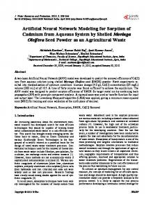
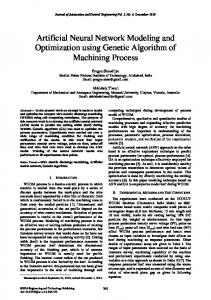
Figure 2 shows schematically the concept of system identification. Once the system identification model is known, the freeway traffic system identification problem is to find a set of parameters such that when the bounded inputs uj(k) are presented to both the system and the identification model, the outputs yˆj(k + 1) of the identification model will approximate the outputs yj(k + 1) of the system. This may be achieved by minimizing the total error between yˆj(k + 1) and yj(k + 1), for example, minimize

∆t ρ j ( k + 1) = ρ j ( k ) + (λ q − λ j q j + rj − s j ) λ j ∆ x j j −1 j −1

( 7)

v j ( k + 1) = v j ( k ) + f [v j −1 ( k ), v j ( k ), ρ j ( k ), ρ j +1 ( k ), . . .]

(8)

q j (k ) = v j (k ) * ρ j (k )

( 9)

∑ eTk e k ∀k

where ek = yˆj(k) – yj(k).

SELECTION OF TRAFFIC FLOW MODELS FOR TRAFFIC SYSTEM IDENTIFICATION

where k j ∆t ∆xj

E=

= = = =

time index; section index, as shown in Figure 1; time increment; length of jth section;

FIGURE 1

Section of freeway.

To study the feasibility of the proposed neural network approach, the higher-order continuum model given by Equations 3–6 is used to simulate the traffic system. There are several realizations of the

112

Paper No. CS7092

TRANSPORTATION RESEARCH RECORD 1588

The term −

δT rj ( k )v j ( k ) ∆ j λ j [ρ j ( k ) + K ]

accounts for ramp merging effects, and − ηφ

FIGURE 2

T λ j − λ j +1 ρ j ( k ) 2 v (k ) ∆j λj ρcr j

for lane drop effects, where η = 0 if λj ≤ λj+1 and η = 1 otherwise. The equilibrium speed above is

System identification.

  ρ  ue (ρ j ) = v f exp − 0.5 j    ρcr    momentum equation given by Chen et al. (6 ); notably, the models of Payne (12) and of Philips (13). Payne’s momentum equation has the following form: µ  ∂ρ dv ∂v 1 = − v − (v − ve ) − dt ∂x T ρT  ∂x 

(12)

where µ and T are parameters and ve is equilibrium speed. On the basis of earlier work by Prigogine (14), Philips developed a family of Boltzman-type statistical traffic models (14–16). One of the Philips models has the following momentum equation: 1  dP ∂ρ ∂v ∂v = − v − λ(v − ve ) −     ∂t ∂x ρ  dρ  ∂x 

(13)

where v ve(ρ) λ(ρ) P(ρ)

= = = =

mean speed, equilibrium speed-density relation, delay coefficient, and traffic pressure function.

Papageorgiou et al. (17) added to Payne’s model a lane drop term and a term that takes account of merging effects in the presence of entry ramps. The resulting discrete momentum equation is T v j ( k + 1) = v j ( k ) + {ue [ρ j ( k )] − v j ( k )} τ µT ρ j +1 ( k ) − ρ j ( k ) T + v j ( k )[v j −1 ( k ) − v j ( k )] − ∆j τ∆ j ρ j ( k ) + K δT rj ( k )v j ( k ) T λ j − λ j +1 ρ j ( k ) 2 v (k ) − − ηφ ∆ j λ j [ρ j ( k ) + K ] ∆j λj ρcr j where k j ∆ λ v ρ r ρcr T, µ, τ, η, φ, δ, K

= = = = = = = = =

time index, freeway section index, section length, number of lanes in a freeway section, speed, density, ramp entry rate, critical density, and constant parameters.

(14)

(15)

where vf is the free-flow speed on a freeway. The aforementioned dynamic traffic models, particularly Payne’s model, appear to be the most realistic models developed (2) and have been used by a number of researchers (11,17–19) in freeway traffic modeling and control studies. However, it has been reported in some studies that both Payne’s and Philips’ models exhibit instabilities and do not track real traffic data correctly (2,20). It has also been reported that Payne’s model may exhibit poor performance at freeway lane drops (21). A recent study (22) indicates that using some numerical schemes can improve the performance of Payne’s model at bottleneck situations, but these schemes do not address the problems that may be inherent in the formulation of the model. Papageorgiou’s model tries to overcome the aforementioned problems by adding the two additional terms. The model was calibrated on the basis of real data (23) and successfully implemented for a stretch of freeway in Paris (17 ). Therefore, the authors decided to use Papageorgiou’s model as the system model, along with the parameters provided by Papageorgiou et al. (17 ).

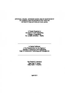
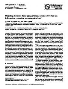
ANN APPROACH FOR TRAFFIC MODELING Figure 3 illustrates the architecture of a multilayer feed-forward neural network. It consists of an input layer of K neurons, one hidden layer of M1 neurons, and another hidden layer of M2 neurons, and an output layer of N neurons. The input layer and first hidden layer are connected by a set of a weights W1, the two hidden layers are connected by a set of weights W2, and the second hidden layer and output layer are connected by a set of weights W3. The inputoutput relationship of this neural network can be described by the following equation: Y = Φ{W3Φ[W2 Φ(W1U + θ1 ) + θ2 ] + θ3}

(16)

where Φ = nonlinear operator, normally a sigmoid type function such as Φ(x) = α/[1 + exp(–x)]; U = input vector; θ1, θ2, θ3 = vectors of thresholds for first hidden layer, second hidden layer, and output layer, respectively.

Zhang et al.

Paper No. CS7092

FIGURE 3

ANN structure. FIGURE 4

Because of the operator’s nonlinearity and the network’s multilayer structure, this type of network can perform highly nonlinear mappings. The weight matrices W1, W2, and W3 and threshold vectors θ1, θ2, and θ3 are adjusted by a learning rule called backpropagation, which is a gradient descent method to minimize the output error with respect to the weights and thresholds (3). In this application, the inputs and outputs of the network are determined according to the traffic flow model used. There are two dynamic equations to be modeled in the traffic flow system. Equation 7 is linear with respect to its inputs [qj–1, qj, rj, sj]. A simple twolayer feed-forward network can capture such a linear relationship, and so the authors do not use a neural network to learn this relationship. Their focus is on the nonlinear, dynamic relationship given in Equation 6 specifically, its realization given by Equation 14. The input vector u(k) to this neural network is [vj–1(k), vj(k), ρj(k), ρj+1(k),

FIGURE 5

113

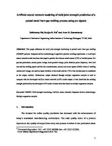
Freeway configuration for neural network training.

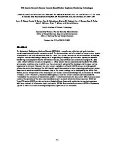
Traffic system identification by neural networks.

rj(k)] and the output vector yˆ (k + 1) = [vj(k + 1)]. As a result, the number of neurons in the input layer is K = 5, and in the output layer N = 1. The learning process is depicted in Figure 4. Inputs are presented to both the traffic flow model based on Equation 14 and the neural network model. The output produced by both models is compared, and the error is fed back to the neural network model, which updates its weights and thresholds on the basis of the backpropagation learning rule. Once the neural network is trained, it should be able to produce outputs that are close to those of the traffic model. To teach the neural network model the relationship given in Equation 14, the authors developed a macroscopic simulation based on Papageorgiou’s model. The results of the simulation are then fed to the neural network. A hypothetical freeway section shown in Figure 5 was used for this study.

114

Paper No. CS7092

TRANSPORTATION RESEARCH RECORD 1588

The freeway section is mostly four lanes, with two lane drops. Each section is 0.5 km long. The simulation time increment T is 15 sec. The boundary conditions are defined by assuming that the speed and density of the beginning section are identical to those of its immediately downstream section, and that the end section is free of congestion during the whole period. The parameters present in Equation 14 are taken from Papageorgiou et al. (17 ). They are follows: vf = 90 km / hr; ρcr = 37.3 veh/km/lane; µ = 35 km2/hr; τ = 36 sec; φ = 2, δ = 0.8; K = 13 veh/km. The system was first initialized to moderate traffic conditions. Then various traffic conditions were generated by varying the ramp volumes and generating random incidents. The entry ramp volume was a random variable that ranged from 120 to 1,800 vehicles per hour. The exit ramp volume was determined by a diversion factor that varied randomly from 0.05 to 0.20 (although the exit ramp volume was limited to not exceed the average freeway volume per lane). It was assumed that incident occurrence followed a Poisson distribution. The distributions of incident duration and number of lanes blocked were estimated. By generating random inputs, the authors attempted to cover the whole input and output space and establish the nonlinear mapping between inputs and outputs. In normal practice, the inputs and outputs to a neural network are scaled to the range of [0,1] or [–1, + 1]. Because a mappingpreserving transformation for a nonlinear relationship is difficult to find, the authors have not scaled their inputs and outputs to avoid distorting the original relationship. During the training process, the authors experimented with the number of hidden neurons. The results were compared with (M1, M2) = (5,5), (10,10), and (20,20) and no significant difference in the network performance was found. However, increasing the number of hidden neurons increases computational time, thus it was decided to use five neurons in each of the two hidden layers, M1 = M2 = 5. The neural network model was trained for 10 million iterations based on the traffic states of Sections 5,6,7,8, and 9. Those five sec-

FIGURE 6

tions were chosen because they had different geometrical features and were less influenced by the boundary conditions. Computationally, it required about 6 hr to complete the 10 million iteration training on a SUN SPARC IPX computer. But once the network was trained, it took much less than 1 sec to simulate 1 hr of traffic for a single section on the same computer, which means that the ANN model can simulate 1 hr of traffic for 60 sections [about 15 mi (24 km)] in less than 1 min.

TEST RESULTS Once the neural network was trained, it was applied to Sections 6, 7, and 8 under different traffic conditions for performance evaluation. These traffic conditions included two demand patterns for the four entry ramps (each demand pattern applied to all the entry ramps, but the magnitude of demand at each ramp may vary), and one incident. The output of the neural network model was compared against that of Papageorgiou’s model, and the relative errors were plotted. The following three test cases are illustrative of the network’s capabilities.

Demand Pattern 1: Entry Ramp Volume Is Step Function In this case the entry ramp demand pattern in Figure 6 was presented to both the neural network and Papageorgiou’s model, for the freeway section. The speed patterns for the three Sections 6, 7, and 8 are shown in the top halves of Figures 7, 8, and 9. The relative errors are shown at the bottom of Figures 7, 8, and 9. These results show that the output from the neural network model [y(k + 1)] closely matches that of Papageorgiou’s model [y d (k + 1)]. Except at a few points, the relative error is within 5 percent. It is noted that higher errors normally appear at either the lowest or the highest speed. This is probably due to not enough

Entry ramp Demand Pattern 1 (step function).

Zhang et al.

FIGURE 7 Speed (top) and error (bottom) for Section 6 (Demand Pattern 1).

data in these ranges being generated and presented during the training process.

Demand Pattern 2: Entry Ramp Volume Is Random with a Trend In this case, the ramp demand pattern in Figure 10 was presented to both the neural network model and Papageorgiou’s model. The results are depicted in Figures 11, 12, and 13. The neural network model obtained better results for Sections 7 and 8 than Section 6, although all the results appear to be satisfactory. The results clearly show that the neural network model captures the nonlinearity embedded in Papageorgiou’s model.

Incident Conditions The authors created an incident that blocked two lanes at Section 7 for 10 min, with the ramp input pattern as shown in Figure 14. The network was tested based on data from Section 6, which is immediately upstream of the incident section. The traffic volume of Section

Paper No. CS7092

115

FIGURE 8 Speed (top) and error (bottom) for Section 7 (Demand Pattern 1).

6 is shown in Figure 15. The test results are shown in Figure 16. The neural network model followed the rapid drop in speed created by the incident closely. CONCLUSIONS In this paper the authors presented the development of a multilayer feed-forward ANN model to address the freeway traffic system identification problem. The solution of this problem is viewed as an essential element in an effort to build an improved freeway traffic flow model for the purpose of developing real-time predictive control strategies for dynamic traffic systems. To study the initial feasibility of the proposed neural network approach for traffic system identification, a three-layer feed-forward neural network model has been developed to emulate an improved version of a well-known higher-order continuum traffic model. Simulation results show that the proposed ANN model not only captures the traffic dynamics of the higher-order continuum traffic model quite closely, but also is computationally efficient for real-time implementation. Future research will attempt to attain similar levels of performance using real traffic data.

FIGURE 9 Speed (top) and error (bottom) for Section 8 (Demand Pattern 1). FIGURE 11 Speed (top) and error (bottom) for Section 6 (Demand Pattern 2).

FIGURE 10

Entry ramp Demand Pattern 2.

FIGURE 12

Speed (left) and error (right) for Section 7 (Demand Pattern 2).

FIGURE 13

Speed (left) and error (right ) for Section 8 (Demand Pattern 2).

FIGURE 14

Entry ramp Demand Pattern 3 (with incident).

118

Paper No. CS7092

TRANSPORTATION RESEARCH RECORD 1588

FIGURE 15

Mainline average volume (per lane) on Section 6.

ACKNOWLEDGMENTS

REFERENCES

The research reported in this paper was supported by the California Department of Transportation and the National Science Foundation.

1. Traffic Control Systems Handbook. Publication LP-123. ITE, Washington, D.C., 1985. 2. Derzko, N. A., A. J. Ugge, and E. R. Case. Evaluation of Dynamic Freeway Flow Model by Using Field Data. In Transportation Research Record 905, TRB, National Research Council, Washington, D.C., 1983, pp. 52–60. 3. Rumelhart, D. E., G. E. Hinton, and R. J. Williams. Parallel Distributed Processing, Vol. I. MIT Press, Cambridge, Mass., 1986. 4. Lo, Z. P., and B. Bavarian. A Neural Piecewise Linear Classifier for Pattern Classification. Proc., International Joint Neural Network Conference, Vol. 1, 1991, pp. 264–268. 5. Ritchie, S. G., M. Kaseko, and B. Bavarian. Development of an Intelligent System for Automated Pavement Evaluation. In Transportation Research Record 1311, TRB, National Research Council, Washington, D.C., 1991, pp. 112–119. 6. Cheu, R. L., S. G. Ritchie, W. W. Recker, and B. Bavarian. Investigation of a Neural Network Model for Freeway Incident Detection. In Artificial Intelligence and Civil and Structural Engineering (B. H. V. Topping, ed.), Civil-Comp Press, 1991, pp. 267–274. 7. Ritchie, S. G., R. L. Cheu, and W. W. Recker. Freeway Incident Detection Using Artificial Neural Networks. Proc., International Conference on A.I. Applications in Transportation Engineering (S. G. Ritchie and C. Hendrickson, eds.), San Buenaventura, Calif., 1992. 8. Kaseko, M., and S. G. Ritchie. A Neural Network-Based Methodology for Automated Distress Classification of Pavement Images. Proc., International Conference on A.I. Applications in Transportation Engineering (S. G. Ritchie and C. Hendrickson, eds.), San Buenaventura, Calif., 1992. 9. Lighthill, M. J., and G. B. Whitham. On Kinematic Waves: II. A Theory of Traffic Flow on Long Crowded Roads. Proc., Royal Society, London, Series A, Vol. No. 229, 1178, 1955, pp. 317–345. 10. Michalopoulos, P. G., D. Beskos, and Y. Yamauchi. Multilane Traffic Flow Dynamics: Some Macroscopic Considerations. Transportation Research B, Vol. 18B, No. 4/5, 1984, pp. 377–395. 11. Papageorgiou, M. Applications of Automatic Control Concepts to Traffic Flow Modeling and Control. Springer-Verlag, 1983. 12. Payne, H. J. Models of Freeway Traffic and Control. Simulation Councils Proceedings Series: Mathematical Models of Public Systems, Vol. 1, No. 1 (G. A. Bekey, ed.), 1971. 13. Phillips, W. F. A Kinetic Model for Traffic Flow with Continuum Implications. Transportation Planning and Technology, Vol. 5, 1979, pp. 131–138. 14. Prigogine, I. A Boltzmann-Like Approach to Statistical Theory of Traffic Flow. In Theory of Traffic Flow (R. Herman, ed.), Elsevier, Amsterdam, the Netherlands, 1961, pp. 158–164. 15. Phillips, W. F. Kinetic Model for Traffic Flow. Report DOT/RSPD/ DPB/50-77/17. U.S. Department of Transportation, 1977. 16. Phillips, W. F. A New Continuum Model for Traffic Flow. Utah State University, Logan, 1979. 17. Papageorgiou, M., J. Blosseville, and H. Hadj-Salem. Modeling and Real-Time Control of Traffic Flow on the Southern Part of Boulevard

FIGURE 16 Speed (top) and error (bottom) for Section 6 (incident situations).

Zhang et al.

18. 19. 20.

21.

Peripherique in Paris: Part I: Modeling. Transportation Research A, Vol. 24A, No. 5, 1990, pp. 345–359. Payne, H. J. FREFLO: A Macroscopic Simulation Model of Freeway Traffic. In Transportation Research Record 722, TRB, National Research Council, Washington, D.C., 1979, pp. 68–75. Zhang, H. A Real-Time Decision-Support System for Freeway Management and Control. M.S. thesis. Department of Civil Engineering, University of California, Irvine, 1992. Hauer, E., and V. F. Hurdle. Discussion of FREFLO: A Macroscopic Simulation Model of Freeway Traffic. In Transportation Research Record 722, TRB, National Research Council, Washington, D.C., 1979, pp. 75–77. Cremer, M., and A. D. May. An Extended Traffic Flow Model for Inner Urban Freeways. Preprints, 5th IFAC/IFIP/IFORS International Con-

Paper No. CS7092

119

ference on Control in Transportation Systems, Vienna, Austria, 1986, pp. 383–388. 22. Leo, C. J., and R. L. Pretty. Numerical Simulations of Macroscopic Continuum Traffic Models. Transportation Research B, 26B, No. 3, 1992, pp. 207–220. 23. Cremer, M., and M. Papageorgiou. Parameter Identification for a Traffic Flow Model. Automatica, 1981, pp. 17, 837–843. The contents of this paper reflect the views of the authors, who are responsible for the facts and the accuracy of the data presented herein. The contents do not necessarily reflect the official views or policies of the state of California. This paper does not constitute a standard, specification, or regulation. Publication of this paper sponsored by Committee on Artificial Intelligence.