He received a BSc. with first class honors in. Computer Science from the University of Dundee in 1991, and an MSc. in Knowledge-. Based Systems (Intelligent ...
Making Reinforcement Learning Work on Real Robots
by William Donald Smart B.Sc., University of Dundee, 1991 M.Sc., University of Edinburgh, 1992 Sc.M., Brown University, 1996
A dissertation submitted in partial fulfillment of the requirements for the Degree of Doctor of Philosophy in the Department of Computer Science at Brown University
Providence, Rhode Island May 2002
c Copyright 2002 by William Donald Smart
This dissertation by William Donald Smart is accepted in its present form by the Department of Computer Science as satisfying the dissertation requirement for the degree of Doctor of Philosophy.
Date Leslie Pack Kaelbling, Director
Recommended to the Graduate Council
Date Thomas Dean, Reader
Date Andrew W. Moore, Reader Carnegie Mellon University
Approved by the Graduate Council
Date Peder J. Estrup Dean of the Graduate School and Research
iii
Vita Bill Smart was born in Dundee, Scotland in 1969, and spent the first 18 years of his life in the city of Brechin, Scotland. He received a BSc. with first class honors in Computer Science from the University of Dundee in 1991, and an MSc. in KnowledgeBased Systems (Intelligent Robotics) from the University of Edinburgh in 1992. He then spent a year and a half as a Research Assistant in the Microcenter (now the Department of Applied Computing) at the University of Dundee, working on intelligent user interfaces. Following that, he had short appointments as a visiting researcher, funded under the European Community ESPRIT SMART initiative, at Trinity College Dublin, Republic of Ireland and at the Universidade de Coimbra, Portugal. In 1994 he moved to the United States to begin graduate work at Brown University, where he was awarded an Sc.M in Computer Science in 1996. When last sighted, he was living in St. Louis, Missouri.
iv
Acknowledgements My parents, Bill and Chrissie have, over the years, shown an amount of patience that is hard for me to fathom. They consistently gave me the freedom to chart my own path and stood by me, even when I started raving about working with robots. Without their support none of this would have been possible. Amy Montevaldo first planted the idea of robotics in my head by leaving a copy of Smithsonian magazine within reach. In many ways, this dissertation is the direct result and owes its existence to her. I am forever in her debt for her kindness, encouragement and friendship. My advisor, Leslie Pack Kaelbling suffered questions, deadline slippage, robot disasters and uncountable other mishaps with tolerance and amazingly good humor. Her advice and guidance have been beyond compare, and I hope that some of her insight is reflected in this work. Mark Abbott and the various members of the Brown University Hapkido club kept me sane during my time at Brown. The chance to hide from the world during training, and the friendship of my fellow martial artists sustained me through some difficult times. Jim Kurien started me on the road to being “robot guy” soon after my arrival at Brown, with seemingly infinite insight into how to solve intractable systems problems. Tony Cassandra, Hagit Shatkay, Kee-Eung Kim and Manos Renieris were the best officemates that I could have wished for, and taught me many things about graduate student life that are not found in books. Finally, I cannot adequately express my gratitude to Cindy Grimm, who has tolerated me throughout the work that led to this dissertation. Without her, you would not be reading this. v
This work was supported in part by DARPA under grant number DABT63-991-0012, in part by the NSF in conjunction with DARPA under grant number IRI9312395, and in part by the NSF under grant number IRI-9453383.
vi
For my grandmother, Isabella.
vii
Contents List of Tables
xii
List of Figures
xiii
List of Algorithms
xvi
1 Introduction
1
1.1
Major Goal and Assumptions . . . . . . . . . . . . . . . . . . . . . .
1
1.2
Outline of the Dissertation . . . . . . . . . . . . . . . . . . . . . . . .
2
2 Learning on Robots
3
2.1
Assumptions . . . . . . . . . . . . . . . . . . . . . . . . . . . . . . . .
3
2.2
Problems . . . . . . . . . . . . . . . . . . . . . . . . . . . . . . . . . .
5
2.2.1
Unknown Control Policy . . . . . . . . . . . . . . . . . . . . .
5
2.2.2
Continuous States and Actions . . . . . . . . . . . . . . . . .
6
2.2.3
Lack of Training Data . . . . . . . . . . . . . . . . . . . . . .
8
2.2.4
Initial Lack of Knowledge . . . . . . . . . . . . . . . . . . . .
8
2.2.5
Time Constraints . . . . . . . . . . . . . . . . . . . . . . . . .
9
2.3
Related Work . . . . . . . . . . . . . . . . . . . . . . . . . . . . . . .
10
2.4
Solutions . . . . . . . . . . . . . . . . . . . . . . . . . . . . . . . . . .
12
3 Reinforcement Learning
13
3.1
Reinforcement Learning . . . . . . . . . . . . . . . . . . . . . . . . .
13
3.2
Algorithms . . . . . . . . . . . . . . . . . . . . . . . . . . . . . . . . .
16
3.2.1
TD(λ) . . . . . . . . . . . . . . . . . . . . . . . . . . . . . . .
16
3.2.2
Q-Learning . . . . . . . . . . . . . . . . . . . . . . . . . . . .
17
viii
3.2.3
SARSA . . . . . . . . . . . . . . . . . . . . . . . . . . . . . .
18
3.3
Related Work . . . . . . . . . . . . . . . . . . . . . . . . . . . . . . .
18
3.4
Which Algorithm Should We Use? . . . . . . . . . . . . . . . . . . . .
20
3.5
Hidden State . . . . . . . . . . . . . . . . . . . . . . . . . . . . . . .
20
3.5.1
Q-Learning Exploration Strategies . . . . . . . . . . . . . . . .
22
3.5.2
Q-Learning Modifications . . . . . . . . . . . . . . . . . . . .
23
4 Value-Function Approximation
26
4.1
Why Function Approximation? . . . . . . . . . . . . . . . . . . . . .
26
4.2
Problems with Value-Function Approximation . . . . . . . . . . . . .
28
4.3
Related Work . . . . . . . . . . . . . . . . . . . . . . . . . . . . . . .
29
4.4
Choosing a Learning Algorithm . . . . . . . . . . . . . . . . . . . . .
31
4.4.1
Global Models . . . . . . . . . . . . . . . . . . . . . . . . . . .
32
4.4.2
Artificial Neural Networks . . . . . . . . . . . . . . . . . . . .
32
4.4.3
CMACs . . . . . . . . . . . . . . . . . . . . . . . . . . . . . .
33
4.4.4
Instance-Based Algorithms . . . . . . . . . . . . . . . . . . . .
35
Locally Weighted Regression . . . . . . . . . . . . . . . . . . . . . . .
35
4.5.1
LWR Kernel Functions . . . . . . . . . . . . . . . . . . . . . .
39
4.5.2
LWR Distance Metrics . . . . . . . . . . . . . . . . . . . . . .
42
4.5.3
How Does LWR Work? . . . . . . . . . . . . . . . . . . . . . .
43
The Hedger Algorithm . . . . . . . . . . . . . . . . . . . . . . . . .
44
4.6.1
Making LWR More Robust
. . . . . . . . . . . . . . . . . . .
45
4.6.2
Making LWR More Efficient . . . . . . . . . . . . . . . . . . .
46
4.6.3
Making LWR More Reliable . . . . . . . . . . . . . . . . . . .
51
4.6.4
Putting it All Together . . . . . . . . . . . . . . . . . . . . . .
54
Computational Improvements to Hedger . . . . . . . . . . . . . . .
57
4.7.1
Limiting Prediction Set Size . . . . . . . . . . . . . . . . . . .
58
4.7.2
Automatic Bandwidth Selection . . . . . . . . . . . . . . . . .
59
4.7.3
Limiting the Storage Space . . . . . . . . . . . . . . . . . . . .
61
4.7.4
Off-line and Parallel Optimizations . . . . . . . . . . . . . . .
61
Picking the Best Action . . . . . . . . . . . . . . . . . . . . . . . . .
62
4.5
4.6
4.7
4.8
ix
5 Initial Knowledge and Efficient Data Use 5.1
64
Why Initial Knowledge Matters . . . . . . . . . . . . . . . . . . . . .
64
5.1.1
Why Sparse Rewards? . . . . . . . . . . . . . . . . . . . . . .
65
5.2
Related Work . . . . . . . . . . . . . . . . . . . . . . . . . . . . . . .
67
5.3
The JAQL Reinforcement Learning Framework . . . . . . . . . . . .
69
5.3.1
The Reward Function . . . . . . . . . . . . . . . . . . . . . . .
70
5.3.2
The Supplied Control Policy . . . . . . . . . . . . . . . . . . .
71
5.3.3
The Reinforcement Learner . . . . . . . . . . . . . . . . . . .
72
JAQL Learning Phases . . . . . . . . . . . . . . . . . . . . . . . . .
73
5.4.1
The First Learning Phase . . . . . . . . . . . . . . . . . . . .
73
5.4.2
The Second Learning Phase . . . . . . . . . . . . . . . . . . .
74
Other Elements of the Framework . . . . . . . . . . . . . . . . . . . .
75
5.5.1
Exploration Strategy . . . . . . . . . . . . . . . . . . . . . . .
75
5.5.2
Reverse Experience Cache . . . . . . . . . . . . . . . . . . . .
76
5.5.3
“Show-and-Tell” Learning . . . . . . . . . . . . . . . . . . . .
76
5.4
5.5
6 Algorithm Feature Effects 6.1
78
Evaluating the Features . . . . . . . . . . . . . . . . . . . . . . . . .
78
6.1.1
Evaluation Experiments . . . . . . . . . . . . . . . . . . . . .
80
6.2
Individual Feature Evaluation Results . . . . . . . . . . . . . . . . . .
81
6.3
Multiple Feature Evaluation Results . . . . . . . . . . . . . . . . . . .
85
6.4
Example Trajectories . . . . . . . . . . . . . . . . . . . . . . . . . . .
87
7 Experimental Results 7.1
90
Mountain-Car . . . . . . . . . . . . . . . . . . . . . . . . . . . . . . .
90
7.1.1
Basic Results . . . . . . . . . . . . . . . . . . . . . . . . . . .
90
7.2
Line-Car . . . . . . . . . . . . . . . . . . . . . . . . . . . . . . . . . .
98
7.3
Corridor-Following . . . . . . . . . . . . . . . . . . . . . . . . . . . . 100
7.4
7.3.1
Using an Example Policy . . . . . . . . . . . . . . . . . . . . . 103
7.3.2
Using Direct Control . . . . . . . . . . . . . . . . . . . . . . . 105
Obstacle Avoidance . . . . . . . . . . . . . . . . . . . . . . . . . . . . 107 7.4.1
No Obstacles . . . . . . . . . . . . . . . . . . . . . . . . . . . 109
7.4.2
Without Example Trajectories . . . . . . . . . . . . . . . . . . 112 x
7.4.3
One Obstacle . . . . . . . . . . . . . . . . . . . . . . . . . . . 114
8 Contributions and Further Work
119
8.1
Contributions . . . . . . . . . . . . . . . . . . . . . . . . . . . . . . . 119
8.2
Further Work . . . . . . . . . . . . . . . . . . . . . . . . . . . . . . . 124
A Reinforcement Learning Test Domains
128
A.1 Mountain-Car . . . . . . . . . . . . . . . . . . . . . . . . . . . . . . . 128 A.2 Line-Car . . . . . . . . . . . . . . . . . . . . . . . . . . . . . . . . . . 129 B The Robot
131
B.1 Locomotion System . . . . . . . . . . . . . . . . . . . . . . . . . . . . 131 B.2 Sensor Systems . . . . . . . . . . . . . . . . . . . . . . . . . . . . . . 132 B.3 Computer Hardware and Software Systems . . . . . . . . . . . . . . . 132 C Computing Input Features from Raw Sensor Information
135
C.1 Detecting Corridors . . . . . . . . . . . . . . . . . . . . . . . . . . . . 135 C.2 Detecting Obstacles . . . . . . . . . . . . . . . . . . . . . . . . . . . . 136 Bibliography
138
xi
List of Tables 6.1
Performance effects of individual Hedger and JAQL features. . . .
7.1
Tabular Q-learning, random policy and simple fixed policy results for the mountain-car domain without a velocity penalty. . . . . . . . . .
7.2
82
91
Final performance of the three function approximators on the mountaincar task. . . . . . . . . . . . . . . . . . . . . . . . . . . . . . . . . . .
96
7.3
Final performances for the line-car task, after 50 training runs. . . . . 100
7.4
Successful simulated runs with no example trajectories. . . . . . . . . 112
xii
List of Figures 2.1
The basic robot model. . . . . . . . . . . . . . . . . . . . . . . . . . .
4
2.2
An example of poor state discretization. . . . . . . . . . . . . . . . .
6
3.1
The basic reinforcement learning model. . . . . . . . . . . . . . . . .
14
4.1
A simple CMAC architecture. . . . . . . . . . . . . . . . . . . . . . .
34
4.2
Fitting a line with linear regression and locally weighted regression. .
38
4.3
Gaussian kernel functions with different bandwidths. . . . . . . . . .
39
4.4
Function used by Schaal and Atkeson.
. . . . . . . . . . . . . . . . .
40
4.5
LWR approximations using different bandwidth values. . . . . . . . .
41
4.6
Fitted lines using LWR and two different weights for extreme points.
43
4.7
Intercept values of the line fitted with LWR as extreme point weight varies. . . . . . . . . . . . . . . . . . . . . . . . . . . . . . . . . . . .
44
4.8
kd-tree lookup complications. . . . . . . . . . . . . . . . . . . . . . .
49
4.9
Hidden extrapolation with LWR. . . . . . . . . . . . . . . . . . . . .
51
4.10 Two-dimensional elliptic hull. . . . . . . . . . . . . . . . . . . . . . .
52
4.11 Elliptic hull failure. . . . . . . . . . . . . . . . . . . . . . . . . . . . .
53
4.12 Typical relationship of MSE to bandwidth for LWR. . . . . . . . . . .
60
5.1
The basic robot control model. . . . . . . . . . . . . . . . . . . . . . .
69
5.2
The learning system. . . . . . . . . . . . . . . . . . . . . . . . . . . .
72
5.3
JAQL phase one learning. . . . . . . . . . . . . . . . . . . . . . . . .
73
5.4
JAQL phase two learning. . . . . . . . . . . . . . . . . . . . . . . . .
74
6.1
Effects of Hedger and JAQL features on total reward. . . . . . . .
82
xiii
6.2
Effects of Hedger and JAQL features on average number of steps to reach the goal. . . . . . . . . . . . . . . . . . . . . . . . . . . . . . . .
6.3
83
Effects of Hedger and JAQL features on the number of successful evaluation runs. . . . . . . . . . . . . . . . . . . . . . . . . . . . . . .
84
6.4
Effects of local averaging with IVH checking and region updating. . .
86
6.5
Effects of the reverse experience cache with IVH checking and region updating. . . . . . . . . . . . . . . . . . . . . . . . . . . . . . . . . .
87
6.6
Performance with and without supplied example trajectories. . . . . .
88
7.1
Performance on the mountain-car task using a CMAC for value-function approximation. . . . . . . . . . . . . . . . . . . . . . . . . . . . . . .
7.2
Performance on the mountain-car task, with an action penalty, using a CMAC for value-function approximation. . . . . . . . . . . . . . . .
7.3
94
Percentage of non-default predictions made by Hedger on the mountaincar task. . . . . . . . . . . . . . . . . . . . . . . . . . . . . . . . . . .
7.6
93
Performance on the mountain-car task using Hedger for value-function approximation. . . . . . . . . . . . . . . . . . . . . . . . . . . . . . .
7.5
93
Performance on the mountain-car task using locally weighted averaging for value-function approximation. . . . . . . . . . . . . . . . . . . . .
7.4
92
95
Performance comparison between LWA and JAQL on the mountain-car task. . . . . . . . . . . . . . . . . . . . . . . . . . . . . . . . . . . . .
97
7.7
Performance in the early stages of learning on the mountain-car task.
98
7.8
Performance on the line-car task using JAQL. . . . . . . . . . . . . .
99
7.9
The corridor-following task, showing two input features. . . . . . . . . 101
7.10 Calculation of the angle input feature for the corridor-following task.
103
7.11 Performance on the corridor-following task, with phase one training directed by an example policy. . . . . . . . . . . . . . . . . . . . . . . 104 7.12 Performance on the corridor-following task, with phase one training directed by a human with a joystick. . . . . . . . . . . . . . . . . . . 106 7.13 Two example supplied trajectories for phase one training, generated by direct joystick control. . . . . . . . . . . . . . . . . . . . . . . . . . 107 7.14 The obstacle avoidance task. . . . . . . . . . . . . . . . . . . . . . . . 108 7.15 The obstacle avoidance task input features. . . . . . . . . . . . . . . . 108 xiv
7.16 Average number of steps to the goal for the obstacle avoidance task with no obstacles. . . . . . . . . . . . . . . . . . . . . . . . . . . . . . 110 7.17 Typical trajectories during learning for the obstacle avoidance task with no obstacles. . . . . . . . . . . . . . . . . . . . . . . . . . . . . . 111 7.18 Average performance of successful runs for the the simulated homing task. . . . . . . . . . . . . . . . . . . . . . . . . . . . . . . . . . . . . 113 7.19 Number of successful evaluation runs (out of 10) for the obstacle avoidance task with one obstacle. . . . . . . . . . . . . . . . . . . . . . . . 115 7.20 Average number of steps to the goal for successful runs of the obstacle avoidance task with one obstacle. . . . . . . . . . . . . . . . . . . . . 116 7.21 Action values with goal state directly ahead while clear (left) and blocked (right) early in learning. . . . . . . . . . . . . . . . . . . . . . 116 7.22 Rotational velocity as a function of distance to an object directly ahead.117 7.23 Greedy action as a function of bearing to an obstacle. . . . . . . . . . 118 A.1 The mountain-car test domain. . . . . . . . . . . . . . . . . . . . . . 128 A.2 The line-car test domain. . . . . . . . . . . . . . . . . . . . . . . . . . 130 B.1 Synchronous drive locomotion system. . . . . . . . . . . . . . . . . . 132 B.2 The control framework. . . . . . . . . . . . . . . . . . . . . . . . . . . 134
xv
List of Algorithms 1
LWR prediction . . . . . . . . . . . . . . . . . . . . . . . . . . . . . .
36
2
LWR prediction with automatic ridge parameter selection . . . . . . .
45
3
LWR prediction with k nearest points . . . . . . . . . . . . . . . . . .
47
4
kd-tree insertion . . . . . . . . . . . . . . . . . . . . . . . . . . . . . .
48
5
kd-tree leaf node splitting . . . . . . . . . . . . . . . . . . . . . . . .
48
6
kd-tree lookup . . . . . . . . . . . . . . . . . . . . . . . . . . . . . . .
50
7
Hedger prediction . . . . . . . . . . . . . . . . . . . . . . . . . . . .
54
8
Hedger training . . . . . . . . . . . . . . . . . . . . . . . . . . . . .
55
9
Finding the greedy action . . . . . . . . . . . . . . . . . . . . . . . .
63
10
Obstacle detection. . . . . . . . . . . . . . . . . . . . . . . . . . . . . 137
xvi
Chapter 1 Introduction Programming robots is hard. Even for simple tasks, it is often difficult to specify in detail how the robot should accomplish them. Robot control code is typically full of constants and “magic numbers”. These numbers must be painstakingly set for each environment that the robot must operate in. The idea of having a robot learn how to act, rather than having to be told explicitly, is appealing. It seems easier and more intuitive for the programmer to provide the high-level specification of what the robot should do, and let it learn the fine details of exactly how to do it. Unfortunately, getting a robot to learn effectively is also hard. This dissertation describes one possible approach to implementing an effective learning system on a real, physical robot, operating in an unaltered environment. Before we begin discussing the details of learning on robots, however, we will explicitly set down the goal of this work, and also the assumptions that we are making.
1.1
Major Goal and Assumptions
The major goal of this work is to provide a framework that makes the use of reinforcement learning techniques on mobile robot effective. Throughout this dissertation, we try to take a practical view of learning on robots. What we mean by this is that, in general, we are only interested in using learning on a mobile robot if it is “better” than using a hand-coded solution. We have two definitions of better: Better: Learning creates a more efficient, or more elegant, solution than a reasonably 1
2 experienced programmer could, in roughly the same amount of time. Faster: Learning produces a solution of comparable efficiency, or elegance, in a shorter time that a reasonably experienced programmer could. So, in essence, we are interested in using learning as a tool to produce mobile robot control code. We assume that our goal is to produce good control policies for a mobile robot operating in an unaltered environment. We also assume that the robot has sufficient sensory capabilities to detect all of the relevant features that it needs to complete the task.
1.2
Outline of the Dissertation
We begin this dissertation with a discussion of learning on real, physical robots in chapter 2. We then go on to introduce the specific learning paradigm, reinforcement learning, that we will be using in chapter 3. In this chapter, we also discuss the shortcomings of this paradigm, in light of our chosen domain. In the following two chapters, we propose solutions for these problems and introduce Hedger, our main reinforcement learning algorithm and JAQL, our framework for using this algorithm for learning on robots. Chapter 6 shows the effectiveness of the individual features of Hedger and JAQL, and looks at how they effect overall performance. We then go on to provide experimental results for JAQL on two simulated and two real robot tasks in chapter 7. Finally, chapter 8 summarizes the contributions made by this dissertation, discusses their relevance and suggests fruitful directions for further work.
Chapter 2 Learning on Robots We are interested in learning control policies for a real robot, operating in an unaltered environment. We want to be able to perform the learning on-line, as the robot interacts with its environment. This poses some unique problems not often encountered in other machine learning domains. In this chapter we begin by discussing the assumptions that we make about the robot, the tasks to be learned and the environment. We then introduce and discuss the problems that must be addressed before an effective learning system can be implemented.
2.1
Assumptions
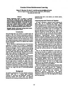
We assume that our robot exists in a world, W, which can be summarized by a (possibly infinite) set of states, S. The robot can make observations from a set, O, of projections of the states in S. Based on these observations, it can take one of a (possibly infinite) set of actions, A, which affect the world stochastically. We also assume that the world is sampled at discrete time steps and that there exists a particular task, T , that we are trying to accomplish. This is shown graphically in figure 2.1. Our goal, then, is to create a mapping from observations to actions that accomplishes the task at hand as efficiently as possible. Such a mapping is known as an action policy for the task T , denoted by πT : O → A. 3
4
S W
O A
Figure 2.1: The basic robot model. If there is no ambiguity about the task, we will generally omit the T subscript and refer to the action policy simply as π. Thus, at every time step, t, the robot makes an observation of the current state of the world, ot ∈ O (corresponding to st ), and generates an appropriate action, at ∈ A, according to its action policy, π at = π(ot ). Taking an action, at , causes the state of the world to change from st to st+1 , with a corresponding new observation, Ot+1 . Note that the observation, ot , can be augmented with the robot’s own internal state, allowing for control policies with persistent memory in addition to those which are purely reactive. In this work, we assume that we are interested in learning a good control policy online, while the robot is interacting with the world. Such interaction is the only way in which we can gather information about the consequences of our actions. Specifically, we do not assume that we have an accurate model of the dynamics of the robot system or a simulator of it.
5
2.2
Problems
Now that we have stated out assumptions about the problem, we can go on to discuss some of the difficulties that must be overcome in order to implement a useful learning system on a real robot.
2.2.1
Unknown Control Policy
A reasonable approach to learning on robots would seem to be to supply a set of training examples consisting of observation-action pairs (oi , ai ) and to use a supervised learning algorithm to learn the underlying mapping. This learned mapping could then be used as the control policy, generalizing to previously unseen observations. There are a number of problems with this approach, however. Supervised learning algorithms attempt to learn the mapping that they are given (embodied in the training examples). This means that, unless we want the system to learn a sub-standard control policy, we must supply the correct action in every training point. If we know the best way to accomplish the task, then it makes sense to simply implement a solution and forget about learning. It is also very possible that we might not know the “best” action to take in every possible situation. Even if we do know a reasonable solution, we might not be able to express it effectively in terms that the robot can use. It is a very different thing, for example, to know how to walk down a corridor than it is to program a robot to do it. Robots are controlled in terms of motor speeds and sensor readings; these are often not intuitive measures for a human programmer. There are also problems associated with the distribution of the training data points. Supervised learning algorithms can generally only make predictions that interpolated from their training data points. If asked to make a prediction that extrapolates from the training points, the results may be unpredictable. This means that not only do we have to know the optimal policy, but we need to know it over the entire observation space. If we can analytically generate appropriate observation-action pairs to train a supervised learner, is there any point in using learning? If we can get good performance by programming the robot, then it might be better to avoid learning. Using a supervised learning approach assumes that we know the “best” control policy for the
6 Goal Position
0.0 (a) (b)
0.25
1 1
0.5
2 2
0.75
3 3
1.0
4 4
5
Figure 2.2: An example of poor state discretization. robot, at least partially. The learning algorithm will try to learn the mapping embodied by the training examples. If the strategy used to generate these examples is suboptimal, the learning algorithm cannot improve on it, and the final learned policy will reflect this. Even if we supply training data that represents the optimal control policy, supervised learning algorithms introduce an approximation error when they make predictions. Although this error might be small, it still introduces an amount of non-optimality and uncertainty into the final learned policy. Our learning method should not rely on knowing a good control policy, and should be able to use suboptimal policies to learn better ones.
2.2.2
Continuous States and Actions
Often robot sensor and actuator values are discretized into finite sets O and A. This can be a reasonable thing to do if the discretization follows the natural resolution of the devices. However, many quantities are inherently continuous with a fine resolution that leads to many discrete states. Even if they can be discretized meaningfully, it might not be readily apparent how best to do it for a given task. Incorrect discretizations can limit the final form of the learned control policy, making it impossible to learn the optimal policy. If we discretize coarsely, we risk aggregating states that do not belong together. If we discretize finely, we often end up with an unmanageably huge state or action space. Figure 2.2 gives an example state discretization leading to a poor final policy. The goal is to bring the vehicle to the center position (x = 0.5).
7 The policy for this is obvious.
π(x) =
x < 0.5 drive right
x = 0.5 halt
x > 0.5 drive left
.
If we discretize the state space into an even number of states, we never have a stable state at the goal. Figure 2.2a shows a discretization with 4 states. This gives the following policy.
π(s) =
1 drive right
3 drive left
2 drive right 4 drive left
In general, the system will oscillate between states 2 and 3, never stopping at the actual goal. If we divide the state space up into an odd number of states, things are slightly better. Figure 2.2b shows a discretization with 5 states. The resulting policy is
π(s) =
1 drive right 2 drive right 3 halt
.
4 drive left 5 drive left
Although this policy causes the vehicle to halt close to the goal state, it is not guaranteed to halt at the goal. If we made the state discretizations smaller, it would be possible to get arbitrarily close to the goal before stopping. However, we would also have an arbitrarily large number of states to deal with. The problem with large numbers of states is compounded when more than one continuous quantity is involved. This is especially true when we are dealing with several continuous sensors. For example, consider a robot with 24 sonar sensors, each returning a value in the range 0 to 32,000. If we discretize each sensor into two states, close and far, thresholding at some appropriate value, we end up with 224 states. Even with such a coarse discretization, this is an unmanageable number of states. This is known as the “curse of dimensionality”.
8 Our learning method should be able to cope with continuous state and action spaces without needing to discretize them. It should be able to generalize in a reasonable way from previously seen examples to novel ones.
2.2.3
Lack of Training Data
Since we are generating data by interacting with the real world, the rate at which we get new training points is limited. Robot sensors often have an inherent maximum sampling rate. Even “instantaneous” sensors, such as vision systems, require time to process the raw data into something useful. Additionally, the world itself changes at a certain rate. In a typical office environment, for example, it is unlikely that any object will be traveling faster than about two meters per second. Sensors which sample extremely quickly will simply generate many training points that are almost identical. We are interested in learning on-line, while the robot is interacting with the world. This means that we cannot wait until we have a large batch of training examples before we begin learning. Our learning system must learn aggressively, and be able to make reasonable predictions based on only a few training points. It must also be able to use what data points it does have efficiently, extracting as much information from them as possible, and generalizing between similar observations when appropriate.
2.2.4
Initial Lack of Knowledge
Many learning systems attempt to learn starting with no initial knowledge. Although this is appealing, it introduces special problems when working with real robots. Initially, if the learning system knows nothing about the environment, it is forced to act more-or-less arbitrarily.1 This is not a real problem in simulated domains, where arbitrary restarts are possible, and huge amounts of (simulated) experience can be gathered cheaply. However, when controlling a real robot it can prove to be catastrophic. Since each control action physically moves the robot, a bad choice can cause it to run into something. This can damage the environment or the robot itself, possibly causing it to stop functioning. Since the robot is a mechanical device, with 1
The system can employ a systematic exploration policy but, for the domains in which we are interested, this is not very practical.
9 inertia and momentum, quickly changing commands tend to be “averaged out” by its mechanical systems. For example, ordering the robot to travel full speed forwards for 0.1 seconds, then backwards for 0.1 seconds repeatedly will have no net effect. Because of the short time for the commands, inertia, slack in the gear trains, and similar phenomena will “absorb” the motion commands. Even if the robot is able to move beyond this initial stage, it will be making what amounts to a random walk through its state space until it learns something about the environment. The chances of this random behavior accomplishing anything useful are likely to be very small indeed. In order for the learning system to be effective, we need to provide some sort of bias, to give it some idea of how to act initially and how to begin to make progress towards the goal. How best to include this bias, how much to supply and how much the learning system should rely on it is a difficult question. Adding insufficient or incorrect bias might doom the learning system to failure. Incorrect bias is an especially important problem, since the programmers who supply the bias are subject to errors in judgment and faulty assumptions about the robot and its environment. Our learning system must be robust in the face of this sort of programmer error, while still being able to use prior knowledge in some way.
2.2.5
Time Constraints
We are interested in learning on-line, while the robot is interacting with the world. Although computers are continually becoming faster, the amount of computation that we can apply to learning is limited. This is especially important when we are using the learned control policy to control the robot. We must be able to make control action choices at an appropriate rate to allow us to function safely in the world. Although this time constraint does not seem like a great restriction, it precludes the use of learning algorithms that take a long time to learn, such as genetic algorithms [45]. Genetic algorithms could learn a good policy overnight, working on stored data. However, for the purposes of this dissertation, we are interested in learning policies as the robot interacts with the world. A related issue is the total amount of time that it takes to learn a control policy.
10 If it takes longer to learn a policy than it would take to explicitly design and conventionally debug one with similar performance, the usefulness of learning is called into question.
2.3
Related Work
The idea of applying learning techniques to mobile robotics is certainly not a new one. There have been several successful implementations of learning on robots reported in the literature. Mahadevan [60] summarizes a number of possible approaches to performing learning on robots. He argues that robot learning is hard because of sensor noise, stochastic actions, the need for an on-line, real-time response and the generally limited amount of training time available. Mahadevan also identifies several areas that learning could be profitably applied on a mobile robot. These area are control knowledge, environment models and sensor-effector models. Although there is currently much interest in all of these areas, especially in map-building and use, we will concentrate on learning for control, since that is the principal focus of this dissertation. Pomerleau [81] overcame the problems of supplying good training data to learn a steering policy for a small truck. A human driver operated the vehicle during the training phase, with the learning system recording the observations and the steering actions made. These observation-action pairs were then used to train a neural network. This side-stepped the problem of having to generate valid training data; the system generated it automatically by observing the human driver. Most drivers tended to stay in the middle of the road, however, leading to a poor sampling of data points in certain parts of the observation space. Pomerleau overcame this by generating additional training examples based on the those actually observed and a geometric knowledge of the sensors and environment. Although the system performed very well, Pomerleau’s work assumes a detailed knowledge of the environment that we do not have in this work. One approach to robot learning is to attempt to learn the inverse kinematics of the task from observation, then use this model to plan a good policy. Schaal and Atkeson [91] use a non-parametric learning technique to learn the dynamics of a devil-sticking
11 robot. They use task-specific knowledge to create an appropriate state space for learning, and then attempt to learn the inverse kinematics in this space. They report successful learning after less than 100 training runs, with the resulting policy capable of sustaining the juggling motion for up to 100 hits. In an extension of their previous work, Atkeson and Schaal [10, 90] use human demonstration to learn a pendulum swing-up task. Two versions of this task were attempted. The easier task is simply swinging the pendulum to an upright position. The more difficult task is to keep the pendulum balanced in this upright position. They describe experiments using both a detailed model of the system dynamics, as well as a non-parametric approach. Both approaches were able to learn the easier of the two tasks, with the parametric approach learning more quickly. However, on the harder task, neither approach could reliably learn to perform the task reliably. For the parameterized approach Atkeson and Schaal attribute this failure to a mismatch between the idealized models being used and the actual dynamics of the system. For the non-parametric approach, they suggest that the state space might not contain all relevant inputs, and cannot cope with the hidden state introduced into the system. They note that “simply mimicking the demonstrated human hand motion is not adequate to perform the pendulum swing up task”, and that learning often finds a reasonable solution quickly, but is often slow to converge to the optimal policy. Other researchers have also explored the area of learning by demonstration. In its most basic form, this results in a human guiding the robot through a sequence of motions that are simply memorized and replayed. This is the preferred method for many assembly and manufacturing tasks using manipulators. However, as Atkeson and Schaal allude to, this is only useful if we know exactly what the robot must do every time. This is fine for applications such as spot-welding, where the robot is simply a repetitive automaton, but it is not adequate for more “intelligent” applications. An alternative is to allow the robot to observe another agent performing the task, and to learn a good control policy from that. This has become known as learning by imitation and has been used for a variety of tasks, including learning assembly strategies in a blocks world [55], the “peg-in-the-hole” insertion task [50], and path-following using another robot as the demonstrator [36]. Bakker and Kuniyoshi [13] give an overview of research in this area. One of the major problems with this approach is in mapping
12 the actions of another agent (possible with a different morphology) to actions of the robot’s own body. One approach to overcome the difficulty in learning complex tasks is robot shaping [38]. In this, the robot is started off close to the goal state, and begins by learning a very simple, constrained version of the task. Once this is achieved, the starting state is moved further from the goal, and learning is resumed. The task is made more and more difficult in stages, allowing the robot to learn incrementally, until the actual starting point of the task is reached. A summary of approaches to robot shaping is given by Perkins and Hayes [80]. Learning based on positive and negative rewards from the environment is another popular approach. Maes and Brooks [59] describe a six-legged robot that learns to sequence its gait by associating immediate positive and negative rewards with action preconditions. Mahadevan and Connell [61] give a detailed report of using reinforcement learning techniques to train a real robot perform a simple box-pushing task. The robot learns to perform better than a hand-designed policy, but is supplied with a good a priori decomposition of the task and carefully trained on each sub-task. Lin [56] also uses reinforcement learning with a neural network to learn a simple navigation task. Asada et al. [7] uses discretization of the state space, based on domain knowledge, to learn offensive strategies for robot soccer. Using reinforcement learning on mobile robots is the main topic of this dissertation, and we will return to the use of this technique in section 3.3.
2.4
Solutions
In this chapter, we have introduced some of the major problems that must be solved before we can successfully implement a learning system on a real robot. The remainder of this dissertation offers some possible solutions to these problems. We begin by introducing reinforcement learning, a learning paradigm that will enable us to overcome the problems discussed in section 2.2.1.
Chapter 3 Reinforcement Learning In this section we introduce reinforcement learning (RL), an unsupervised learning paradigm that is well suited for learning on robots. RL techniques learn directly from empirical experiences of the world. We begin by presenting the basic RL framework and then discuss some popular algorithms and techniques.
3.1
Reinforcement Learning
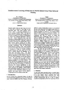
The basic reinforcement learning model is shown in figure 3.1. It is similar to the model in figure 2.1, except that it includes an additional input from the environment to the learning agent. This is an immediate reward from the environment, representing a measure of how good the last action was. The model of interaction with the environment is the same as before; the agent makes an observation of the environment, ot , and selects an action, at . It then performs this action, resulting in a transition to a new state, st+1 , with its corresponding observation, ot+1 and a reward, rt+1 . Our ultimate goal is to learn a policy, π : O → A, mapping observations to actions. If we assume that the world is fully observable, i.e. ot = st , this is equivalent to learning the policy π : S → A, mapping states to actions. In the real world, we must often deal with hidden state, where a single observation maps to two (or more) underlying states of the world. For clarity, we will ignore hidden state for the moment, returning to it in section 3.5. 13
14
W S R
O A
Figure 3.1: The basic reinforcement learning model. When learning control policies, we must be able to evaluate them with respect to each other. In RL the evaluation metric is some function of the rewards received by the agent. The most obvious metric, the sum of all rewards over the life of the robot, ∞ X
rt ,
t=0
is generally not used. For agents with infinite lifetimes, all possible sequences of rewards would sum to infinity. This is not the case for agents with a finite lifetime, however. In this case, the obvious metric turns into the finite horizon measure, k X
rt .
t=0
This measure sums the rewards over some finite number, k, of time steps. Average case, k 1X rt , k→∞ k t=0
lim
extends this extends this by using the average reward received over the whole lifetime (or learning run) of the agent. The infinite horizon discounted measure, ∞ X t=0
γ t rt ,
15 uses a discount factor, 0 ≤ γ ≤ 1, to give more weight to rewards that happen sooner in time (and, thus, have a smaller value for t). If we set γ to be zero, then we obtain the one-step greedy policy; the best action is the one that gives the greatest immediate reward. Values greater than zero reflect how much we are concerned with actions that happen further in the future. In this dissertation, we will be using an infinite horizon discounted sum of rewards as our measure of policy optimality, mostly because the theoretical aspects are better understood. One justification for the infinite horizon metric is that if the future is uncertain (if there is stochasticity in the environment), rewards that we may get in the future should mean less to us that rewards the we do get now. The further into the future the potential rewards are, the more uncertainty that they are subject to, and the less weight they should have. An alternative interpretation of the infinite horizon discounted measure is that it is the same as the finite horizon measure when we are uncertain about where the horizon is. A discount factor of γ corresponds to a chance of 1 − γ of reaching the horizon on any given time step. RL problems are typically cast as Markov decision processes (MDPs). In an MDP there is a finite set of states, S, a finite set of actions, A, and time is discrete. The reward function R:S×A→R returns an immediate measure of how good an action was. The resulting state, st+1 , is dependent on the transition function T : S × A → Π (S) which returns a probability distribution over possible next states. An important property of MDPs is that these state transitions depend only on the last state and action. This is known as the Markov property. The problem, then, is to generate a policy, π : S → A, based on these immediate rewards that maximizes our expected long-term reward measure. If we know the functions T and R then we can define an optimal value function, V ∗ , over states: " ∗
V (s) = max R(s, a) + γ a
# X
0
∗
0
T (s, a, s ) V (s ) .
s0
This function assigns a value to each state which is the best immediate reward that we can get for any action from that state added to the optimal value from each of
16 the possible resulting states, weighted by their probability. If we know this function, then we can define the optimal policy, π ∗ by simply selecting the action, a, that gives the maximum value: #
" ∗
π (s) = arg max R(s, a) + γ
X
a
0
∗
0
T (s, a, s ) V (s ) .
s0
There are well-understood methods for computing V ∗ (such as value iteration and policy iteration, see Sutton and Barto [98]), which lead to a simple procedure for learning the optimal value function, and hence the optimal policy. First we learn (or are given) models of the environment, which correspond to the T and R functions. This lets us calculate the optimal value function, and from this the optimal policy. However, learning good models often requires a large amount of data and might be difficult in a potentially changing world. Instead of learning T and R, however, we can incrementally learn the optimal value function directly. In the next section, we describe three well-known algorithms that attempt to iterative approximate the optimal value function.
3.2
Algorithms
The three algorithms that we present in this section learn value functions incrementally, based on experiences with the world. These experiences are states, s, actions, a, and rewards, r. All experiences are indexed with the time at which they occurred, e.g. (st , at , st+1 ). All of the algorithms store their value functions in a tabular form and assume discrete states and actions.
3.2.1
TD(λ)
Sutton’s Temporal Difference (TD(0)) algorithm [95] iteratively learns a value function for states, V (s), based on state-transitions and rewards, (st , rt+1 , st+1 ). Starting with a random value for each state, it iterative updates the value-function approximation according to the following update rule: V (st ) ← (1 − α)V (st ) + α (rt+1 + γV (st+1 )) .
17 There are two parameters; a learning rate, α, and a discount factor, γ. The learning rate controls how much we change the current estimate of V (s) based on each new experience. The update rule can also be written in the following form, which better shows its connections to the following two algorithms: V (st ) ← V (st ) + α (rt+1 + γV (st+1 ) − V (st )) . A more general version of the TD(0) algorithm is TD(λ). In this the rule above is changed to V (st ) ← V (st ) + α (rt+1 + γV (st+1 ) − V (st )) et (st ) , and it is applied to every state, rather than just the one that was most recently visited. Each state is updated according to it’s eligibility, et (st ). All eligibilities start out at zero and are updated on each time step according to
et (s) =
γλet−1 (s)
if s 6= st
γλet−1 (s) + 1 if s = st
,
where γ is the discount factor, and λ is the eligibility decay parameter. This means that eligibilities decay over time, unless they are visited (s = st ), in which case, they are incremented by 1. TD learns the value function for a fixed policy. It can be combined with a policylearner to get what is known as an actor-critic or an adaptive heuristic critic system [14]. This alternates between learning the value function for the current policy, and modifying the policy based on the learned value function.
3.2.2
Q-Learning
Q-learning [111] learns a state-action value function, known as the Q-function, based on experiences with the world. This function, Q(s, a), reflects how good it is, in a long-term sense that depends on the evaluation measure, to take action a from states. It uses 4-tuples (st , at , rt+1 , st+1 ) to iteratively update an approximation to the optimal Q-function, Q∗ (s, a) = R (s, a) + γ
X s0
T (s, a, s) max Q∗ (s, a0 ) . 0 a
18 Once the optimal value function is known, the optimal policy, π ∗ (s) can be easily calculated: π ∗ (s) = arg max Q∗ (s, a) . a
Since the policy is fixed with respect to time, we can omit the time indexes. The Q-values can be approximated incrementally online, effectively learning the policy and the value function at the same time. Starting with random values, the approximation is updated according to �
0
�
Q (st+1 , a ) − Q (st , at ) Q (st , at ) ← Q (st , at ) + α rt+1 + γ max 0 a
In the limit, it has been shown [111] that this iterated approximation for Q(s, a) will converge to Q∗ (s, a), giving us the optimal policy, under some reasonable conditions (as as the learning rate, α, decaying appropriately).
3.2.3
SARSA
SARSA [88] is similar to Q-learning in that it attempts to learn the state-action value function, Q∗ (s, a). The main difference between SARSA and Q-learning, however, is in the incremental update function. SARSA takes a 5-tuple, (st , at , rt+1 , st+1 , at+1 ), of experience, rather than the 4-tuple that Q-learning uses. The additional element, at+1 , is the action taken from the resulting state, st+1 , according to the current control policy. This removes the maximization from the update rule, which becomes Q (s, a) ← Q (st , at ) + α (rt+1 + Q (st+1 , at+1 ) − Q (st , at )) . Just like TD, SARSA learns the value for a fixed policy and must be combined with policy-learning component in order to make a complete RL system.
3.3
Related Work
The reinforcement learning algorithms described above are the direct descendents of work done in the field of dynamic programming [16, 19, 84]. More specifically, the three algorithms presented above are closely related the Value Iteration algorithm [16, 19], used to iteratively determine the optimal value function.
19 TD(λ) was introduced by Sutton [95], and was proved to converge by several researchers [77, 33, 105]. An alternative version of the eligibility trace mechanism, where newly visited states get an eligibility of 1, rather than an increment of 1, was proposed by Singh and Sutton [94]. Q-learning was first proposed by Watkins [110, 111]. Eligibility trace methods, similar to those for TD(λ) were proposed by Watkins [110], with a slightly different formulation described by Peng and Williams [77, 79], although they have not been proved to be convergent in the general case. Comprehensive comparison experiments between these two approaches were described by Rummery [87]. SARSA is due to Rummery [88], and can also be formulated with an eligibility mechanism. Reinforcement learning techniques have had some notable successes in the past decade. Two of the most notable are described here. Tesauro’s backgammon player TD-Gammon [100, 99, 101]. used temporal difference methods, a very basic encoding of the state of the board. A more advanced version employed some additional human-designed features, describing aspects of the state of the board, greatly improving performance. Learning was carried out over several months, with the program playing against versions of itself. TD-Gammon learned to play competitively with top-ranked human backgammon players, and was considered one of the best players in the world. Backgammon has a huge number of states, and Tesauro used valuefunction approximation techniques (see section 4) to succeed where a table-based approach would have been infeasible. Crites and Barto used Q-learning in a complex simulated elevator scheduling task [30, 31]. The simulation had four elevators operating in a building with ten floors. The goal was to minimize the average squared waiting time of passengers. Again, the state space was too large for table-based approaches to work, so value-function approximation was used. The final performance was slightly better than the best known algorithm, and twice as good as the controller most frequently used in real elevator systems. Other successful RL applications include large-scale job-shop scheduling [117, 118, 119], cell phone channel allocation [93], and a simplified highway driving task [65]. RL techniques have also been applied to robots for tasks such as box-pushing [61], navigation tasks [56], multi-robot cooperation [64] and robot soccer [7]. Wyatt [116]
20 discusses effective exploration strategies for RL systems on real robots. Good introductions to reinforcement learning techniques can be found in the survey by Kaelbling, Littman and Moore [49], and in the book by Sutton and Barto [98].
3.4
Which Algorithm Should We Use?
The three algorithms presented in section 3.2 have all been shown to be effective in solving a variety of reinforcement learning tasks. However, there is a fundamental difference between Q-learning and the other two that makes it much more appealing for our purposes. The TD and SARSA algorithms are known as on-policy algorithms. The value function that they learn is dependent on the policy that is being followed during learning. Q-learning, on the other hand, is an off-policy algorithm. The learned policy is independent of the policy followed during learning. In fact, Q-learning even works when random training policies are used. Using an off-policy algorithm, such as Q-learning, frees us from worrying about the quality of the policy that we follow during training. As we noted in the previous chapter, we might not know a good policy for the task that we are attempting to learn. Using an on-policy algorithm with an arbitrarily bad training policy might cause us not to learn the optimal policy. Using an off-policy method allows us to avoid this problem. There are still potential problems, however, with the speed of convergence to the optimal policy when using training policies that are not necessarily very good.
3.5
Hidden State
The description of RL, given above, assumes that the world is perfectly observable; the robot can determine the true state of the world accurately. Unfortunately, this is not the case in reality. Robot sensors are notoriously noisy, and give very limited measurements of the world. With this sensor information, we can never be completely sure that our calculation of the state of the world is accurate. This problem is known as partial observability, and can be modeled by a partially observable MDP (POMDP). The solution of POMDPs is much more complicated and problematic than that of
21 MDPs, and is outside the scope of this thesis. By limiting ourselves to MDPs, we are essentially ignoring the problem of hidden state. However, we are using a robot in a real, unaltered environment which most definitely does have hidden state. We cannot directly sense all of the important features of the environment with the sensors that the robot has. To allow us to get around the problem of hidden state, we assume that the robot is supplied with a set of virtual sensors that operate at a more abstract level than the physical sensors do. These virtual sensors will typically use the raw sensor readings and specific domain knowledge to reconstruct some of the important hidden state in the world. Examples of such sensors might be a “middle-of-the-corridor” sensor, that returns the distance to the middle of the corridor that the robot is in, as a percentage of the total corridor width. This virtual sensor might use readings from the laser range-finder, integrated over time, along with geometric knowledge of the structure of corridors. By supplying an appropriate set of such virtual sensors, we can essentially eliminate the problem of hidden state for a given task. The most obvious way to create these virtual sensors is to have a human look at the task and decide what useful inputs for the learning system might be. For some tasks, such as obstacle avoidance, this will be straightforward. However, in deciding what virtual sensors to create and use, we are introducing bias into the learning system. An alternative approach is to use learning to create virtual sensors. In its most basic form, this consists of selecting a minimal useful set of the raw sensors to use for a particular task. This is known as feature subset selection in the statistics literature. There are several standard methods to find minimal subsets of features (corresponding to sensors in our case) that predict the output (the action) well (see, for example, Draper and Smith [39]). Many of these are based on linear regressions and are only effective for relatively small amounts of data and a few features (sensors), due to their computational expense. Much of the feature selection work in the machine learning literature deals with boolean functions. Example solutions include weighting each input and updating these weights when we get the wrong prediction [57], employing heuristics to generate likely subsets using a wrapper approach [5] and using information-theoretic principles to determine relevant inputs [54]. Some work, such as that by Kira and Rendell [52],
22 deals with continuous inputs but still requires the outputs to be binary classifications. There seems to be little or no work dealing with continuous inputs and outputs that is not directly derived from methods described the statistical literature. There has also been some work looking at how to create higher-level features from raw sensor data. De Jong [35] uses shared experiences between agents to learn a grammar that builds on raw sensory input. The concepts represented by this grammar can be seen as corresponding to high-level features that the agents have agreed upon as being useful. Martin [63] uses genetic programming techniques to learn algorithms that extract high-level features from raw camera images.
3.5.1
Q-Learning Exploration Strategies
Q-learning chooses the optimal action for a state based of the value of the Q-function for that state. After executing this action and receiving a reward, the Q-function approximation is updated. If only the best action is chosen (according to the current approximation), it is possible that some actions will never be chosen from some states. This is bad, because we can never be certain of having found the best action from a state unless we have tried them all. It follows that we must have sort of exploration strategy which encourages us to take non-optimal actions in order to gain information about the world. However, if we take too many exploratory actions, our performance will suffer. This is known as the exploration/exploitation problem. Should we explore to find out more about the world, or exploit the knowledge that we already have to choose a good action? There are a number of solutions to this problem proposed in the literature. Perhaps the simplest solution is known as “optimism in the face of uncertainty”. Since Q-learning will converge to the optimal Q-function regardless of the starting Q-value approximations, we are free to choose them arbitrarily. If we set the initial values to be larger than the largest possible Q-value (which can be calculated from the reward function), we encourage exploration. Imagine a particular state, s, with 4 possible actions. The first time we arrive in s, all of the values are the same, so we choose an action, say a1 , arbitrarily. That action causes a state transition and a reward. When we update our approximation of Q(s, a1 ), the new value is guaranteed to be smaller than the original, overestimated value. The next time we encounter
23 state s, the three other actions a2 , a3 and a4 , will all have larger values than a1 , and one of them will be selected. Only when all of the actions have been tried will their actual values become important for selection. Another approach is to select a random action a certain percentage of the time, and the best action otherwise. This is called an �-greedy strategy, when � is the proportion of the time we choose a random action. The parameter, � allows us to tune this exploration strategy, specifying more (� → 1) or less (� → 0) exploration. We may also change the value of � over time, starting with a large value and reducing it as we become more and more certain of our learned policy. A third approach is similar to �-greedy, but attempts to take into account how certain we are that actions are good or bad. It is based on the Boltzmann distribution and is often called Boltzmann exploration or soft-max exploration. At time t, action a is chosen from state s with the following probability. eQ(s,a)/τ Pr (a|s) = X Q(s,a0 )/τ e a0
The parameter τ > 0 is called the temperature. High temperatures cause all actions to have almost equal probability. Low temperatures amplify the differences, making actions with larger Q-values more likely. In the limit, as τ → 0, Boltzmann selection becomes greedy selection. Systems typically start with a high temperature and “cool” as learning progresses, converging to a greedy selection strategy when the Q-function is well-known. It is unclear whether one method of action selection is empirically better than another in the general case. Both have one parameter to set, but it seems that � is conceptually easier to understand and set appropriately than τ .
3.5.2
Q-Learning Modifications
In this section, we cover some modifications and additions to the basic Q-learning algorithm presented above. These are all intended to provide some improvement in learning speed or convergence to the optimal policy. The most basic modification is the attenuation of the learning rate. A common practice is to start with a learning rate, α, set relatively high and to reduce it over
24 time. This is typically done independently for each state action pair. We simply keep a count, cs,a , of how many times that each state-action pair has been previously updated. The effective learning rate, αs,a , is then determined from the initial rate by αs,a =
α . cs,a + 1
The idea behind this is that as we gain more and more knowledge about a certain state-action pair, the less we will have to modify it in response to any particular experience. Attenuating α can cause the Q-function to converge much faster. It might not, however, converge to the optimal function, depending on the distribution of the training experiences. Consider the case where the training experiences can be partitioned into two sets, E1 and E2 , where E1 is the subset of “correct” experiences, and E2 is the subset of “incorrect” ones caused, for example, by gross sensor errors. Typically, |E1 | >> |E2 | and so, with enough training data, the policy calculated from the data in E1 will dominate. If we see many data points from E2 before we see any from E1 , and we are attenuating the learning rate, we might converge to a non-optimal policy. If we see enough points from E2 , the learning rate for many state-action pairs will be sufficiently low that when the data from E1 come in, they have little or no effect. This sort of effect will also be apparent if the domain is non-stationary. If the optimal policy changes over time, this method is not appropriate since, after a sufficient amount of data, it freezes the value function, and the policy implied by it. Dyna [96] is an attempt to make better use of the experiences that we get from the world. The idea is that we record, for every state, all of the actions taken from that state, and their outcomes (the next state that resulted). From this we can estimate the transition function, Tˆ(s, a, s0 ) and average reward for each state-action ˆ a). At each step of learning, we choose k state-action pairs at random from pair, R(s, our recorded list. For each of these pairs, we then update the value function according to !
ˆ (si , ai ) + γ Q (si , ai ) ← Q (si , ai ) + α R
X s0
Tˆ (si , ai , s0 ) max Q (s0 , a0 ) − Q (si , ai ) 0 a
Dyna has been found to reduce the amount of experience needed by a considerable amount, although it has to perform more computation. In domains where computation is cheap compared to experience (as it is when dealing with real robots), this is a good tradeoff.
25 The main problem with Dyna is that it spends computation on arbitrary parts of the state-action space, regardless of whether or not they are “interesting’. Two very similar algorithms which attempt to address this problem are Prioritized Sweeping [71] and Queue-Dyna [78]. Prioritized Sweeping is similar to Dyna, in that it updates state-action pairs based on previously remembered experiences and learned models. However, to focus attention on “interesting” state-action pairs, it assigns a “priority” to each state-action pair. Each time a backup (real or from memory) is performed on a state-action pair, its priority, ps,a , is set to the magnitude of the change in its Q-value. ps,a =
� � α r + γ max Q (s0 , a0 ) − Q (s, a) a0
After each real iteration, we perform k steps of prioritized sweeping updates. We pick the state-action pair with the highest priority and perform an update as in Dyna. This will cause the priority of the pair to change. We then select the new highest priority pair, and so on until we have performed k backups. The effect of prioritized sweeping is to cause state-action pairs which undergo large changes in Q-value to have high priority and receive more attention. Large changes in Q-value probably mean that we do not have a very good approximation of the Q-value for that pair. Note that, since we continually update the priorities for each state-action pair, the attention is focused on successive predecessor states to the most interesting one. Prioritized sweeping has been shown to be even more effective in terms of actual experience required than Dyna in several domains. Queue-Dyna works in a similar manner, ordering the list of state-action pairs to be processed by Dyna.
In this chapter, we have briefly covered the three most common reinforcement learning algorithms and selected one, Q-learning, on which to base our work. The following chapter looks at an important extension to the algorithms presented here; the ability to deal with multi-dimensional continuous state and action spaces.
Chapter 4 Value-Function Approximation In the previous chapter we introduced reinforcement learning and described some common algorithms for learning value-functions. We showed how Q-learning can be used to learn a mapping from state-action pairs to long-term expected value. However, all of the algorithms described assume that states and actions are discrete and that there are a manageable number of them. In this chapter, we look at how to extend Q-learning to deal with large, continuous state spaces where this is not the case.
4.1
Why Function Approximation?
In chapter 3, we discussed how Q-learning can be used to calculate the state-action value-function for a task. This function can be used in combination with one-step lookahead to calculate the optimal policy for the task. The methods presented all assume that the Q-function is explicitly stored in a table, indexed by state and action. However, it is not always possible to represent the Q-function in this manner. When the state or action spaces become very large it may not be possible to explicitly represent all of the possible state-action pairs in memory. If we can usefully generalize across states or actions, then using a function approximator allows us to have a more compact representation of the value function. Even if the state-action space is small enough to be represented explicitly, it may still be too large for the robot to usefully explore. To be sure that we know the best action from every state,
26
27 we must try each possible action from every state more than once.1 If we assume the state can change 50 times each second, then in one hour of experimentation we can visit 180,000 state-action pairs. However, this state-change frequency is extremely optimistic for a real mobile robot, which might have to physically move through space to generate state transitions. Some of the transitions will lead to different states in the continuous space that are not interesting (i.e., too close to each other to matter) from the control point of view. Useful transitions, therefore, will be much slower than the 50Hz suggested. It is also unlikely that state-action pairs will be visited uniformly, so there will actually be much fewer than 180,000 unique pairs actually observed by the learning system. Using a function approximator removes the need to visit every state-action pair, since we can generalize to pairs that we have not yet seen. If the state or action spaces are continuous, we are forced to discretize them in order to use a table-based approach. However, discretization can lead to the inability to learn a good policy and an unmanageable number of states, as discussed in section 2.2.2. It is possible to discretize continuous spaces more cleverly, or to create new, more abstract discrete states for the reinforcement learning system to use. For example, Moore and Atkeson [72] attempt to plan a path from a start region to a goal region in a multidimensional state space using a coarse discretization. When the planning fails, they iteratively increase the resolution in the part of the space where the path planner is having problems. Asada et al. [7] use specific knowledge of the robot soccer domain to transform a camera image into one of a set of discrete states. The discretization is based on the distance and relative orientations of the ball and goal and results in a total of 319 discrete states. Although both of these approaches were successful, in general it requires skill to ensure that the set of abstract states is sufficient to learn the optimal policy. 1
Recent work by Kearns and Singh [51] suggests that for a domain with N states, the near-optimal policy can be computed based on O(N log N ) state-action samples.
28
4.2
Problems with Value-Function Approximation
Using a function approximator to replace the explicit table of Q-values seems to be a reasonable solution to the problems outlined in the previous section. However, there are several new problems to be overcome before we can take this approach with Q-learning. The convergence guarantees for Q-learning [111] generally do not hold when using a function approximator. Boyan and Moore [21] showed that problems can occur even in seemingly benign cases. The main reason for this is that we are iteratively approximating the value-function. Each successive approximation depends on a previous one. Thus, a slight approximation error can quickly be incorporated into the “correct” model. After only a few iterations, the error can become large enough to make the learned approximation worthless. A major problem with using a function approximator is that the state-action space often does not have a straightforward distance metric that makes sense. Some of the elements of the state-action vector refer to states and may reflect raw sensor values, combinations of sensor values or abstract states. Others represent actions and may refer to quantities such as speed, torque or position. Simply applying the standard Euclidean distance metric to these quantities may not be very useful. Specific learning algorithms will be affected by this to different extents, based on how heavily they use an explicit distance metric. Nearest neighbor methods, for example, are very sensitive to the distance metric. Other algorithms, such as feed-forward neural networks, will be affected to a much lesser degree. A related problem is the implicit assumption of continuity between states and actions. If one point in the state-action space is close to another, by whatever distance metric is being used, then they are assumed to be somehow similar, and therefore have similar values. Although this is often true when we are dealing with continuous sensor values, there may be cases where the assumption does not hold. The more we know about the form of the value-function, the less data we need to evaluate it and more compact our representation can be. For example, if we know the parametric form of the function, the job of representing and approximating it becomes almost trivial. However, we generally do not have such detailed knowledge and are forced to use more general function approximation techniques. We discuss
29 the criteria that such a function approximator must satisfy in the next section.
4.3
Related Work
Value-function approximation has a long history in the dynamic programming literature. Bertsekas and Tsitsiklis [20] provide an excellent survey of the state-of-the-art in this area, which they refer to as neurodynamic programming (NDP), because of the use of artificial neural networks as function approximators. However, this work makes certain assumptions that mean it cannot be directly applied to our problem domain. Bertsekas and Tsitsiklis explicitly state that NDP methods often require a huge amount of training data, are very computationally expensive and are designed to be carried out off-line [20, page 8]. In the reinforcement learning setting, Boyan and Moore [21] showed that valuefunction approximation can case problems, even in seemingly easy cases. Sutton [97] provided evidence that these problems could be overcome with a suitable choice of function approximator, and by sampling along trajectories in the state space. Despite the lack of general convergence guarantees, various approaches using gradient descent and neural network techniques[12, 11, 82, 93, 100, 114, 118] have been reported to work on various problem domains. TD with linear gradient-descent function approximation has been shown to converge to the minimal mean squared error solution [33, 107]. Successful implementations using CMACs, radial basis functions and instancebased methods have also been reported [69, 89, 97, 102]. The collection of papers edited by Boyan, Moore and Sutton [23] also gives a good overview of some of the current approaches to value-function approximation. Gordon [46] has shown that a certain class of function approximators can be safely used for VFA. Those function approximators that can be guaranteed not to exaggerate the differences between two target functions can be used safely. That is, if we have two functions f and g and their approximations, fˆ and gˆ, ˆ f (x) − g ˆ (x)
≤ |f (x) − g (x)| .
30 K Several common function approximators, such as locally weighted averaging, knearest neighbor and B`ezier patches satisfy this requirement. Gordon defines a general class of function approximators which he calls “averagers” which satisfy the above condition, and are therefore safe for VFA. These have the property that any approximation is a weighted average of the target values, plus some offset, q fˆ (x) = k +
X
βi f (xi ) .
i
A similar class of function approximators, called interpolative representations, was defined by Tsitsiklis and Van Roy [106]. Although most approaches concentrate on using a function approximator to store the value function, there has been some work on using variable-resolution discretization methods. Variable Resolution Dynamic Programming [70] begins with a coarse discretization of the state space, on which standard dynamic programming techniques can be applied. This discretization is refined in parts of the state space that are deemed to be “important”. The importance of a discretized region is calculated by performing simulations of the task that pass though that state. Moore’s Parti-Game algorithm [72] also starts with a coarse discretization of the state space. The algorithm assumes the availability of a local controller for the system that can be used to make transitions from one discretized cell to another. Shortest-path algorithms can then be used to calculate a trajectory from the start state to the goal. A discretized cell is split into several smaller cells when the original is too coarse to allow good navigation through the environment. Parti-Game’s main failing is in its reliance on local controllers, and the fact that it searches for any solution to a given task, and does not try to find the optimal one. Another related approach was proposed by Munos [75, 76] which again begins with a coarse discretization of the state space and selectively refines this discretization. A cell is split (or not), depending on its influence on other cells, as determined by the dynamics of the system and the discount factor. Cells which have a high influence on goal states tend to be split. This tends to result in many small cells along decision boundaries in the state space. However, the approach assumes that we know the dynamics of the system. Although several successful implementations of VFA have been reported in the literature, they all assume something that we cannot in our problem domain. For
31 this dissertation, we assume that we have no explicit knowledge of the goal states, local controllers are not available and we have no model of the system dynamics. Although, however, one or more of these things will be present and can be used to accelerate learning. For this work, we want to look at the “base case”, where none of them are available. This will give us a lower bound on the sort of learning performance that we can expect. We spend the rest of this chapter describing a value-function approximation algorithm that avoids the assumptions made by much of the previous work.
4.4
Choosing a Learning Algorithm
The basis of any value-function approximator is the supervised learning algorithm used to actually represent the function. There are several requirements for such a learning algorithm. Incremental We are interested in on-line learning, so the algorithm must be capable of learning one data point at a time. We should not have to wait until we have a large batch of data points before training the algorithm. Aggressive The algorithm should be capable of producing reasonable predictions based on only a few training points. Since we are learning on-line, we want to use the algorithm to make predictions early on, after only a few training points have been supplied. Confidence Estimates The predictions supplied by the algorithm are used to generate new training points for it. Any error in the original prediction quickly snowballs, causing the learned approximation to become worthless. In addition to providing a prediction for a query point, the algorithm should be able to indicate how confident it is of this prediction. Predictions with low confidence should not be used to create new training instances. Non-destructive Since we will typically be following trajectories through stateaction space, the training point distribution will change over time. The algorithm should not be subject to destructive interference or “forgetting” of old values, in areas of the space not recently visited.
32 We now list some popular choices for value-function approximators and discuss their applicability to our domain in light of these requirements.
4.4.1
Global Models
If we know that the value function has a certain parametric form, then all that we have to do is to estimate the values of these parameters. Traditional regression methods [39, 68] seem like a good choice in this case. The methods are well understood and are easily implemented. We can estimate prediction confidence through the use of several standard statistics. One problem is that regression methods are performed in batch mode, not incrementally, and can become computationally expensive as the number of data points becomes large. Stochastic gradient descent methods are a solution to the batch learning problem. These methods use an estimate of the effects that parameter changes will have on the prediction error to iteratively improve the parameter estimates. The partial derivative of the prediction error with respect to the parameters, along with a learning rate, α, is used to determine how much each of the parameters should be altered. Typically, a rule such as pi ← pi − α
∂E ∂pi
is used, where pi is one of the parameters and E is the error. However, these methods can require many iterations and large amounts of training data in order to converge to a good set of estimates. For most problems, however, the form of the value function is not known. This limits the usefulness of methods relying on global models.
4.4.2
Artificial Neural Networks
Artificial neural networks (ANNs) [48, 86] seem like a natural choice for value-function approximation. They can model arbitrarily complex functions and can make predictions efficiently once trained. However, they do not learn aggressively. It typically takes many training examples, well distributed over the input space before ANNs begin to make reasonable predictions. ANNs are also typically “black box” learners;
33 new training data is incorporated into the model and then discarded. This means that we cannot get a measure of the confidence in a given prediction. ANNs also suffer from the problem of destructive, or catastrophic, interference [66, 85]. Suppose that we learn the value function in one part of the state-action space. We then move to another part of the space and continue learning there. If the originally learned model is not valid in the new part of the space, it will be changed so that it reflects the current training data. This will destroy our previously acquired knowledge about the original part of the space, a phenomenon known as destructive interference. Although there are methods for alleviating this problem [112], none are foolproof. In general, since we are sampling from a trajectory through state-action space (generated by the moving robot), such destructive interference could prove to be a considerable problem. ANNs have been used successfully as value-function approximators in several reinforcement learning systems [20, 93, 100, 118]. However, in all of these applications learning is done off-line, training data is plentiful and well-distributed over the state space and, in most cases, the experiences can be generated in arbitrary order, not being constrained to follow trajectories though the state space. Under these conditions, ANNs are a reasonable choice for value function approximation. However, in our domain, these conditions are rarely (if ever) met.
4.4.3
CMACs
The Cerebellar Model Articulation Controller (CMAC) [2, 3, 4] is another algorithm that has proven to be popular for value-function approximation work. The algorithm splits the input space into a number of overlapping receptive fields, each with an associated response. Any given input will lie within a small number of these fields, known as the activated fields. The response of the CMAC to this input is simply the average response of the activated fields. The sizes of these receptive fields determine how aggressively the CMAC generalizes across the input space. Figure 4.1 illustrates this with a simple CMAC with a two-dimensional input space and four receptive fields. Point A lies only within field 2, so the output would be the response of that field. Point B lies within two receptive fields (2 and 3), and the output is the average of the responses of these fields. Finally, point C lies within all of the fields, so the
34 4 1
C
A
B
3 2
Figure 4.1: A simple CMAC architecture. output is the average of all of the responses. Training is performed in CMACs by presenting an input, xi , and comparing the predicted output, yˆi with the actual one, yi . The responses of all activated fields are then changed according to ∆R = α (yi − yˆi ) , where 0 < α < 1 is a learning rate that determines how aggressively we change to match new examples. The output for a particular point is simply the average of the responses of its activated receptive fields, and this can never be greater than the largest response in the CMAC. Since the responses are determined by the observed outputs, yi , they can never be larger than those values (assuming we initialize the responses with some small, random value). Thus, a CMAC behaves essentially like an averaging function approximator, and therefore satisfies Gordon’s conditions [46] for a convergent valuefunction approximation algorithm. A similar algorithm, multivariate adaptive regression splines (MARS) [43] exists, and can be trained without the gradient descent methods used by CMACs.
35
4.4.4
Instance-Based Algorithms
Instance-based algorithms simply store their training data. When asked to make a prediction, they use the stored points close (according to some distance metric) to the query point to generate a suitable value. For example, the simplest instance-based algorithm, known as 1-Nearest Neighbor [29, 32], returns the value of the stored point closest to the query as a prediction. The computational load of these algorithms is mostly borne during prediction, not during learning. These methods are often called lazy learning algorithms since they postpone their work until it must be done. Instance-based algorithms typically learn aggressively and are able to generate plausible predictions after only a few training samples. They can also use their stored data to estimate the reliability of a new prediction, and do not suffer from destructive interference. However, they do suffer from the computational complexity of making predictions. Since they typically compare the query point to all of the previously seen training points, a naive implementation can have a prediction complexity of O(n) for n training points. Added to this is the complexity of actually making the prediction based on the stored points.
Despite their computational drawbacks, we have chosen an instance-based learning algorithm as the basis of our value-function approximation scheme. In the next section we describe this algorithm and then go on to show how its computational complexity can be tamed.
4.5
Locally Weighted Regression
Locally weighted regression (LWR) [8, 9] is a variation of the standard linear regression technique in which training points close to the query point have more influence over the fitted regression surface. Given a set of training points, linear regression fits the linear model that minimizes squared prediction error over the whole training set. This implicitly assumes that we know the global form of the underlying function that generated the data. LWR, on the other hand, only fits a function locally, without imposing any requirements on the global form.
36 The LWR learning procedure is simply to store every training point. Algorithm 1 shows how predictions are made for a given query point. The training and query Algorithm 1 LWR prediction Input: Set of training examples, {(~x1 , ~y1 ), (~x2 , ~y2 ) . . . (~xn , ~yn )} Query point, ~xq Bandwidth, h Output: Prediction, ~yq 1: Construct a matrix, A, whose lines correspond to the ~ xi s 2: Construct a matrix, b, whose lines correspond to the ~ yi s 3: for each point (~ xi , ~yi ) do 4: di ← distance(~xi , ~xq ) 5: ki ← kernel(di , h) 6: Multiply the ith lines of A and b by ki 7: Perform a linear regression using A and b to get a local model, f (~ x) 8: return ~ yq = f (~xq ) points are assumed to be pairs of real-valued vectors (~x, ~y ). There is one real-valued parameter for the algorithm, h, known as the bandwidth. The algorithm constructs a matrix, A, just as in standard linear regression, where
p 1 2 x1 x1 . . . x 1 1 1 x2 x22 . . . xp2 1
p 1 2 A= x3 x3 . . . x 3 1 . . .. . . .. . . . . .
x1n x2n . . . xpn 1
The rows of A correspond to the ~xi s. Another matrix, b is also constructed, corresponding to the ~yi s,
b=
y11 y21 .. .
y12 y12 .. .
... ... ...
y1q y2q .. .
yn1 yn2 . . . ynq
.
A standard linear regression would then solve Ax = b. However, LWR now goes on to weight the points, so that points close to the query have more influence over
37 the regression. For each data point in the training set, the algorithm calculates that point’s distance from the query point (line 4). A kernel function is then applied to this distance, along with the supplied bandwidth, h, to give a weighting for the training point (line 5). This weighting is then applied to the lines of the A and b matrices. A standard linear regression is then performed using the modified A and b to produce a local model at the query point (line 7). This model is then evaluated that the query point, and the value is returned. In general, for an m-dimensional space, the bandwidth would actually be an mdimensional vector, ~h. This admits the possibility of a different bandwidth value for each of the dimensions. In this dissertation, however, we assume that the bandwidths for all dimensions are the same, ~h = {h, h . . . h}, and simply use the scalar h to represent the bandwidth. LWR calculates a new model for every new query point. This differs from standard regression techniques, which calculate one global model for all possible queries. Although this allows LWR to model more complex functions, it also means that it is significantly more computationally expensive than a single global regression. One way to think about how LWR works is shown in figure 4.2. A standard linear regression attaches springs between the data points and the fitted line. All of the springs have the same strength, and the line shown in figure 4.2(a) is the result. This line is used to answer all queries. Locally weighted regression, on the other hand, fits a new line for each query. It does this by measuring the distance between the query point and each data point, and making the strength of the springs vary with distance. Springs closer to the query point are stronger, those further away are weaker, according to the kernel function. This means that points close to the query have more influence on how the fitted line is placed. This can be seen in figure 4.2(b), where the same data points generate a different fitted line. This line is only used for the particular query point shown. For another query, the spring strengths will be different and a different line will be fit to the data. Algorithm 1 uses two functions, one to calculate the distance from training points to query points, and one to turn this distance into a weighting for the points. In the following sections we look at these functions more closely, and then go on to discuss why LWR actually works.
38
Fitted line
(a) Standard linear regression
Query Point (b) Locally Weighted regression Figure 4.2: Fitting a line with linear regression and locally weighted regression.
39 100
1.0
Weighting
0.8 10
0.6 5
0.4 1
0.2 0.1 0.0
0
2
4 6 Distance to query
8
10
Figure 4.3: Gaussian kernel functions with different bandwidths.
4.5.1
LWR Kernel Functions
The kernel function, used on line 3 of algorithm 1, is used to turn a distance measure into a weighting for each training point. It is parameterized by a bandwidth, h, which controls how quickly the influence of a point drops off with distance from ~xq . A Gaussian, d
2
kernel (d, h) = e−( h ) , is typically used, where d is the distance to the query point and h is the bandwidth. Other kernel functions, such as step functions, are also possible. The only restrictions on the form of kernel functions are kernel (0, h) = 1 kernel (d1 , h) ≥ kernel (d2 , h) , d1 ≤ d2 kernel (d, h) → 0,
.
as d → ∞
The actual shape of the kernel has some effect on the results of the local regression, but these effects are typically small for a wide class of kernel functions [109]. We use a Gaussian kernel because it has infinite extent, and will never assign a zero weight to any data point. For kernel functions which go to zero, it is possible for all training points to be far enough away from the query that they are all weighted to zero. Figure 4.3 shows some example Gaussian kernels and their bandwidths. The bandwidth is a measure of how smooth we think the function to be modeled is. Its value has a significant effect on the outcome of the regression. Large bandwidths produce very smoothed functions, where all of the training points have a similar effect
40
"schaal"
1.4 1.2 1 0.8 0.6 0.4 0.2 0
-1
0 0
x
y
-1
Figure 4.4: Function used by Schaal and Atkeson. on the regression. Small bandwidths tend towards nearest neighbor predictions. As h → ∞ the local regression tends towards a global regression, since each training point will have a weight of 1. We now give an example to illustrate the effects of varying the bandwidth in LWR. The function that we are attempting to learn is one used previously in work by Schaal and Atkeson [92]. The function is shown in figure 4.4 and is given by n
�
�
�
�
�
�
f (x, y) = max exp −10x2 , exp −50y 2 , 1.25 exp −5 x2 + y 2
��o
.
The function consists of two ridges, one narrow and one wider, and a Gaussian bump at the origin. In all of the following examples, we use 500 training points drawn from the input space according to a uniform random distribution. Figure 4.5 shows the models learned with varying bandwidth settings. With very small bandwidths, all points are assigned weights close to zero. This leads to instabilities in the local regressions, and results in a poor fit. With large bandwidths the local regressions take on the character of global regressions since every point is weighted close to 1. Somewhere between these two extremes lies a good choice of bandwidth, where the function is well modeled. Note that in figure 4.5 the function is never particularly well modeled, partly because of the relatively small number of training points and partly because the optimal bandwidth is not shown. Getting a good model of the function hinges on finding this “best” bandwidth, and we will discuss this further in section 4.7.2.
41
Bandwidth 0.001
Bandwidth 0.005 "schaal-0.001"
"schaal-0.005"
1.4 1.2 1 0.8 0.6 0.4 0.2 0
1.4 1.2 1 0.8 0.6 0.4 0.2 0
-1
0
-1
y
0
x
0 x
-1
y
0 -1
Bandwidth 0.01
Bandwidth 0.05 "schaal-0.010"
"schaal-0.050"
1.4 1.2 1 0.8 0.6 0.4 0.2 0
1.4 1.2 1 0.8 0.6 0.4 0.2 0
-1
0 x
-1
y
0
0 x
-1
y
0 -1
. Bandwidth 0.1
Bandwidth 0.5 "schaal-0.100"
"schaal-0.500"
1.4 1.2 1 0.8 0.6 0.4 0.2 0
1.4 1.2 1 0.8 0.6 0.4 0.2 0
-1
0
-1
y
0
x
0 x
-1
0 -1
eps Bandwidth 1
Bandwidth 5 "schaal-1.000"
1.4 1.2 1 0.8 0.6 0.4 0.2 0
"schaal-5.000"
1.4 1.2 1 0.8 0.6 0.4 0.2 0
-1
0 x
0 -1
y
-1
0 x
0
y
-1
Figure 4.5: LWR approximations using different bandwidth values.
y
42
4.5.2
LWR Distance Metrics
LWR uses the distance from the query point to each of the training points as the basis for assigning weights to those points. This means that the choice of distance metric has a large effect on the predictions made. Typically, Euclidean distance is used distance (~p, ~q) =
v u n uX t w2 (p i
i
− qi )2
i=0
where wi is a weight applied to each dimension. If this weight is 1, the standard Euclidean distance is returned. This implicitly assumes that all elements of the vectors being compared have ranges of approximately equal width. If this is not the case, different weights can be used for each dimension. This is equivalent to normalizing all of the ranges before computing the distance. The weights can also be used to emphasize dimensions that are more important than others, and cause them to have more effect on the distance calculation. It should be noted that this distance metric is designed for continuous quantities does not deal well with nominal values. An alternative distance metric is the Minkowski metric [15, pp 71–72], given by distance (~p, ~q) =
n X
!1 r
|xi − yi |
r
.
i=0
Euclidean distance is simply the Minkowski distance with r = 2. The Manhattan, or city-block, distance is Minkowski with r = 1. As r increases, points that are far from each other (in the Euclidean sense) get further away. When viewed in terms of kernel functions, as r increases, far away points are weighted closer and closer to zero. Other, more complex, distance functions are also possible; Wilson [115, chapter 5] gives a summary in terms of instance-based learning algorithms. For the work reported in this dissertation, we will use standard Euclidean distance as our metric. Although it might not be the best metric in every case, we have found empirically that it gives reasonable results. It also has the advantage of being easily interpretable, which will proved to be useful when debugging and testing the algorithms described in this section.
43 6
5
4
y = 3.714286
3
y = 3.2
2
1
0
0
2
4
6
8
10
Figure 4.6: Fitted lines using LWR and two different weights for extreme points.
4.5.3
How Does LWR Work?
How does LWR manage to focus attention around the query point and disregard points that are far from it? A standard linear regression fits a line to a set of data points by minimizing the squared prediction error for each data point, n X
(yi − yˆi )2 ,
i=1
where (xi , yi ) is a training point, and yˆi is the prediction for that point. LWR applies a weight, ki , to each of the training points based on their distance from the query point. Points far away have smaller weights, points closer in have larger weights. This means that we are now minimizing a weighted sum n X
(wi yi − wi yˆi )2 = w12 (y1 − yˆ1 ) + w22 (y2 − yˆ2 ) + . . . + wn2 (yn − yˆn ) .
i=1
Points that have small weights will not play less of a part in the sum of errors, and will thus have less effect on the final fitted line. Figure 4.6 illustrates this with a simple example. There are five data points, (1, 2), (4, 4), (5, 4), (6, 4), and (9, 2). The result of a standard linear regression, where all points have the same weight, is the line y = 3.2. If weight the first and last points half as much as the other three, the line changes to y = 3.714286. This reflects the greater influence of the three middle points. Figure 4.7 shows how the intercept value changes with the relative weights of the two extreme data points. With a weight of
44 4 3.8
Intercept value
3.6 3.4 3.2 3 2.8 2.6 2.4 2.2 2
0
0.5
1
1.5
2
2.5
3
3.5
4
4.5
5
Weight Figure 4.7: Intercept values of the line fitted with LWR as extreme point weight varies. zero, they are ignored. As their weight increases, the intercept of the fitted line gets closer and closer to 2, as they dominate the other three points. Although LWR would never weight distant points more heavily, this helps show the mechanisms at work.
4.6
The Hedger Algorithm
In this section we introduce Hedger, our algorithm for safely approximating the value function. It is based on the LWR learning algorithm and on a modified version of the Q-learning algorithm that was given in section 3.2.2. Before we describe Hedger itself, we will first discuss some modifications to the standard LWR procedure that our algorithm takes advantage of. Although LWR is a good choice for value-function approximation, there are some serious drawbacks. One is related to potential instabilities in fitting the regression model to the training set. Another, and more serious, problem is that LWR requires a huge amount of computation for even moderately large training sets, which must be repeated for each query point. A third problem is due to the fact that we are trying to learn a non-stationary function. We discuss our approaches to solving these problems in the following sections.
45
4.6.1
Making LWR More Robust
There is a potential problem in simply applying algorithm 1 to fit a set of training points. The algorithm uses the training points to construct a set of linear equations which are then solved to calculate the local regression model. If we have many data points far from the query point, many of the coefficients of these scaled equations will be small. This can cause problems with numerical stability, and lead to less wellfitting models. One way to alleviate this problem is known as ridge regression [39, 8]. Instead of solving the original system of equations AX = B, as in algorithm 1, we construct another matrix, Z = AT A + ρI, where ρ is known as the ridge parameter. When this parameter is zero, the solution of ZX = AT B is exactly the same as that of the original system of equations. However, when AT A is close to singular, adding in ρI, for non-zero ρ, typically improves the stability of the computation but introduces a bias into the parameter estimation (since we are not solving the original system of equations any more). Since such a bias is undesirable, we would like to use ridge regression techniques only when we must. When we do use them, we would like to use as small a ridge term as possible to minimize the amount of additional bias introduced. This leads to Algorithm 2. The algorithm tries to fit a reliable surface Algorithm 2 LWR prediction with automatic ridge parameter selection Input: Set of training examples, {(~x1 , ~y1 ), (~x2 , vecy2 ) . . . (~xn , ~yn )} Query point, ~xq Bandwidth, h Output: Prediction, ~yq 1: Assemble A and b and weight their lines, as in algorithm 1 2: ρ ← 10−10 3: Z ← AT A 4: while Z cannot be factored do 5: Z ← AT A + ρI 6: ρ ← 10ρ 7: solve ZX = AT B to get local model f (~ x) 8: return ~ yq = f (~xq ) to the data points, while introducing as little bias as possible. First, we assemble the A and b matrices and weight their lines using the kernel function, as before (line 1).
46 We then set the initial ridge parameter, ρ (line 2) and create a new matrix, Z, from A (line 3). The z matrix is tested to see if it can be successfully factored. If Z is close to singular, it cannot be factored and we must add in a ridge term.2 The initial ridge term is small (line 2), and is gradually increased until we create a Z that can be factored. At this point, we go ahead and complete the prediction as before (lines 7 and 8). This procedure ensures that we make a robust prediction, while at the same time adding as little bias as possible. All future references to LWR in this dissertation implicitly assume that we are using algorithm 2 to provide a robust fitted model. The problem of the matrix AT A being singular is well known in the statistics literature, generally resulting from the use of what is called “unplanned data”, where the experimenter has no direct control over the specific data points being generated (for example, see Draper and Smith [39]). There are a number of possible techniques in the literature for dealing with the problem (of which ridge regression is one), but they often involve the use of domain-specific knowledge or subjective input from the statistician.
4.6.2
Making LWR More Efficient
The greatest drawback to using LWR as a value-function approximator is the computational expense of making queries. Queries have a complexity of O(nd2 + d3 ), for n training points and d dimensional inputs, and using the entire training set to perform the prediction typically requires a massive amount of computation. However, many of the data points used in the regression will have little effect, since they will be far from the query point. If we are willing to tolerate a small additional prediction error, we can simply ignore these low-influence points. Using only a small set of influential training points to perform the prediction will greatly reduce the amount of computation needed to make a prediction. In order to select an appropriate subset of the training points to answer a given query, we select the k points closest to the query point. This can be done simply, as shown in algorithm 3. We compute the distances from the query point to each stored training point, and select the k smallest ones. Using the na¨ıve implementation given in algorithm 3 means finding the k closest 2
Factoring Z is a step in the process of solving the system ZX = AT B.
47 Algorithm 3 LWR prediction with k nearest points Input: Set of training examples, {(~x1 , ~y1 ), (~x2 , ~y2 ) . . . (~xn , ~yn )} Query point, ~xq Set size, k Bandwidth, h Output: Prediction, ~yq 1: for each point (~ xi , ~yi ) do 2: di ← distance(~xi , ~xq ) 3: sort points (~ xi , ~yi ) by di 4: K ← k points with smallest di s 5: return ~ yq = LWR prediction based on K and h points has a complexity of O(n), since we must search through all n stored data points. However, if we store the data points more cleverly, we can avoid having to search through all of them to find those closest to the query point. We use a kdtree[18, 44, 69] to store our data for the nearest neighbor algorithm.3 A kd-tree is a binary tree designed to hold multi-dimensional data. Each internal node of the tree defines an axis-parallel hyperplane in the input space. Data points to the “left” of this plane belong to that point’s left subtree, otherwise they belong to the right subtree. The hyperplane is represented by a split dimension (representing which axis the hyperplane cuts) and a split value (where it cuts the axis). In two dimensions, the kd-tree divides the space into axis-parallel rectangles. The leaf nodes hold small “bags” of data points. This differs from some implementations which store one data point per node, both internal and leaf nodes. Given a set of data points, and assuming identical training and testing distributions, it is possible to build an optimally-balanced kd-tree. However, since we are interested in learning on-line, we are forced to construct the tree one point at a time. The most straightforward approach simply finds the leaf node to which the new point belongs and adds it to the bag for that node. We then perform a test to see if the bag should be split into two smaller bags and a new internal node added to the tree. Currently this decision is based on the size of the bag; once it exceeds a preset size 3
The k in kd-tree is different from the k in k-nearest neighbor. The former refers to the dimensionality of the data, whereas the latter refers to the size of the set used to make a prediction. Unfortunately, both are in common use.
48 limit, it is split. Algorithm 4 shows the insertion procedure in detail. Line 3 checks Algorithm 4 kd-tree insertion Input: Data point, (~x, ~y ) kd-tree, T 1: if T is a leaf node then 2: add (~x, ~y ) to the bag of data 3: if the bag contains too many points then 4: replace T with return value of splitting algorithm 5: else 6: if ~xs < vs then 7: insert (~x, ~y ) in left subtree 8: else 9: insert (~x, ~y ) in right subtree to see if the number of points in the bag of data exceeds the preset limit. If it does, the data in the bag are split between two new nodes, using algorithm 5. The test at Line 6 compares the element of ~x in the split dimension, s, with the split value, vs . If ~xs < vs , the point is to the “left” of the splitting plane and is recursively inserted in the left child. Otherwise it is inserted in the right child. Leaf node splitting is performed by Algorithm 5. The choice of split dimension and value is critical for a Algorithm 5 kd-tree leaf node splitting Input: kd-tree leaf node L Output: New kd-subtree, T 1: create a new internal node, I 2: create two new leaf nodes, Ll and Lr 3: set Ll and Lr to be the left and right children of I, respectively 4: set split dimension and value 5: for all points, (~ xi , ~yi ) in L do 6: insert (~xi , ~yi ) into I 7: return I well-balanced tree. However, since we are incrementally building the tree we must use heuristic methods. Ideally, we would like the leaf nodes in our kd-tree to contain data points that are close to each other in the input space. This will typically make
49 A
B
A B
C
C
Figure 4.8: kd-tree lookup complications. the lookup procedure more efficient. Since leaf nodes cover hyper-rectangular areas of the input space, we would like them to be as “square” as possible. This will tend to minimize the distances between points owned by a given leaf node. In order to accomplish this, we select the dimension that has the most spread out points (within the node to be split) and split it at the mean of the values in the split dimension. It should be noted that there are other methods of incrementally building such trees that guarantee to maintain balance (for example R-trees [47]). We have found, however, that the simple heuristic presented here is sufficient for our purposes. There is one case in which algorithm 5 will fail. If all of the points in the node being split are exactly the same, any choice of splitting dimension and value will result in all of the points being assigned to the same the new child nodes. In this case, we do not perform the split. Instead, we increase the number of points allowed in the node that was to be split, and store the new point there. To find the closest point to a query using a kd-tree, we first find the leaf node that owns the query point. We then compare each of the points in that node with the query point and return the closest. However, there is a problem with this approach. As illustrated in Figure 4.8, it is possible for a point outside of the leaf node to be closer than any inside it. The query point (black dot) is owned by node B. The closest point inside node B is further away than a point in node A. Thus, we need to search node A in addition to node B in order to be sure that we really have the closest point. We accomplish this by keeping track of the distance to the closest point found so far, dclose . If we draw a circle around the query point with a radius of dclose , then we need only consider nodes that intersect this circle. As we find points closer and closer to the query point, the size of this circle will shrink. Eventually, the circle
50 will be totally contained within the area owned by nodes that have been visited. At this point, no further search is necessary. This essentially amounts to performing a depth-first search, guided by the query point, terminating when there is no possibility of finding a training point closer to the query than the current one. This procedure, in its most basic form, is shown in algorithm 6. We first call the algorithm with a Algorithm 6 kd-tree lookup Input: kd-tree, T Query point, ~xq Closest point, (~x, ~y ) Closest distance, dclose Output: Closest stored point, (~x, ~y ) 1: if T is a leaf node then 2: find closest point to ~xq in data bag, (~xc , ~yc ) 3: if dist(~xq , ~xc ) < dclose then 4: (~x, ~y ) ← (~xc , ~yc ) 5: dclose ← dist(~xq , ~xc ) 6: else 7: if ~xq belongs to left subtree of T then 8: perform lookup in left subtree of T 9: perform lookup in right subtree of T 10: else 11: perform lookup in right subtree of T 12: perform lookup in left subtree of T 13: if no possible closer points then 14: return (~x, ~y ) null closest point and dclose = ∞ on the root node of the kd-tree. It then recursively walks down the tree until it reaches a leaf node. At this point, it finds the closest point contained in the leaf node and makes a note of it. We then begin to unwind the recursion, examining the branches of the tree that were not originally taken, operating in the same way as depth-first search. This process continues until the circle centered on the query point, with a radius of dclose lies completely within the current node. At this point, we terminate and return the closest point. A simple extension to algorithm 6 allows us to collect the k nearest points to the query. We keep an ordered list of the k nearest points found so far, and set dclose to
51 1.5
1
Actual 0.5
0
−0.5
Prediction −1
−1.5
0
2
4
6
8
10
Figure 4.9: Hidden extrapolation with LWR. be the distance to the furthest point in this set. Other speedups are also possible, where models are precomputed and the results stored in nodes of the kd-tree. For example, Moore, Schneider and Deng [74] store the results of regressions over subtrees, AT A and AT b, in the root node of that subtree, combining them when a prediction is needed.
4.6.3
Making LWR More Reliable
The final problem with LWR that we need to address is what is known in the statistics literature as hidden extrapolation [17]. Regression models are fitted to minimize error on their training set and are only valid for the area of input space covered by that set. They can only be trusted to interpolate between training points, not to extrapolate beyond them. Figure 4.9 gives an example of the dangers. The local regression was trained on points in the range 0 to 5. In this range, the prediction is very close to the actual curve. However, once we leave this region the prediction quickly diverges from the actual curve. One solution to this problem is to construct a convex hull around the training data and to only answer queries that lie within this hull. The intuition behind this is that queries with the hull will be supported by the training points. However, constructing the convex hull of a set of n points in d dimensional space can be computationally expensive, especially when d is large. De Berg et al. [34] give a randomized algorithm �
�
with an expected running time of Θ nbd/2c , and the best known algorithm, due to �
�
Chan [25] runs in O n log f + (nf )1−1/(bd/2c+1) logO(1) n time, where f is the number of faces in the convex hull. For n points in d dimensions, d + 1 ≤ f ≤ n.
52
Figure 4.10: Two-dimensional elliptic hull. Instead of calculating the exact convex hull around the training points, we can calculate an approximate one instead. Cook [27] calls this structure the independent variable hull (IVH) and suggests that the best compromise of efficiency and safety is a hyper-elliptic hull, arguing that the expense of computing more complex hulls outweighs their predictive benefits. Determining whether a point lies within this hull is straightforward. For a matrix, X, where the rows of X correspond to the training data points, we calculate the hat matrix V = X(X T X)−1 X T . An arbitrary point, ~x, lies within the hull formed by the training points, X, if ~xT (X T X)−1~x ≤ max vii i
where vii are the diagonal elements of V . This quantity represents a weighted measure of the query point’s distance to the center of mass of the training points. The closer to this center the point is, the more we can trust its predicted value. Figure 4.10 shows the hull around a set of two-dimensional points. The computational complexity of calculating the approximate elliptic hull is O(n3 ), and O (d2 ) for determining whether a given point is within the precalculated hull.
53
?
Figure 4.11: Elliptic hull failure. There are many plausible solutions to the problem of hidden extrapolation. Looking at the closest training point to the query, or calculating the local density of training point are two possibilities. For our purposes, however, using the IVH removes the need for a pre-set threshold. A query point is either within the hull, or outside of it. Any queries within the convex hull (the shaded area in figure 4.10) can be trusted; those outside cannot. If we are willing to add a “don’t know” answer to our LWR function approximator, we can greatly improve the overall quality of the predictions. When the k nearest points are collected for the LWR prediction, if the query point falls within the elliptic hull that they define, everything proceeds as normal. If the query is outside of the hull, then we return a “don’t know” answer. There are situations when using any convex hull will not be sufficient, however. Figure 4.11 illustrates one such situation, with an approximate elliptic hull. The data points are arranged in a “C”-shaped region. Drawing a hull around them includes the empty space within the “C”. This is dangerous, since we have no data for this area and cannot safely make predictions for queries within it. If we were to fit a more complex hull around the data points, we could avoid this particular instance of the problem, but it would be easy to find another. In general, using an hyper-elliptic hull is regarded as the best tradeoff between computational expense and prediction safety
54 [27].
4.6.4
Putting it All Together
In this section we describe Hedger, our value-function approximation algorithm. It is based on LWR, augmented with the improvements presented in the previous sections, and a modified version of the Q-learning algorithm presented in section 3.2.2. Algorithm 7 shows the basic Hedger prediction algorithm. States and actions are Algorithm 7 Hedger prediction Input: Set of training examples, S State, s Action, a LWR set size, k LWR bandwidth, h Output: Predicted Q-value, qs,a 1: ~ x ← (s, a) 2: K ← closest k training points to ~ x 3: if we cannot collect k points then 4: qs,a = qdef ault 5: else 6: construct an IVH, H, using points in K 7: if ~x is outside of H then 8: qs,a = qdef ault 9: else 10: qs,a = LWR prediction using ~x, K, and h 11: if qs,a > qmax or qs,a < qmin then 12: qs,a = qdef ault 13: return qs,a assumed to be real-valued vectors. We begin by concatenating the state and action vectors into a compound query vector, ~x (line 1). We then find the k closest points to ~x in the training set S (line 2). If we cannot collect k points (perhaps because it is early in learning), we return the default Q-value. Otherwise, we construct an IVH around these closest points, and test the compound query point against it. If the query is outside of the hull, we do not risk a prediction and return a default Q-value. If the point is within the hull, we go ahead and make an LWR prediction as
55 normal (line 10). If the predicted value is outside of the possible limits for Q-values, then we assume that something has gone wrong and return the default Q-value. The Q-value limits are calculated by the Hedger training algorithm (shown below), and are based on the rewards observed and the discount factor. Only if there are enough training points, the compound query point is within the hull and the predicted value is within the acceptable limits, do we return the actual prediction. Algorithm 7 is designed to make conservative predictions. If there is any doubt about the ability to make a prediction for a given state-action pair, it will return the default Q-value. Algorithm 8 gives the Hedger training algorithm. The algorithm keeps track Algorithm 8 Hedger training Input: Set of training examples, S Initial state, ~st Action, ~at Next state, ~st+1 Reward, rt+1 Learning rate, α Discount factor, γ LWR set size, k LWR bandwidth, h Output: New set of training examples, S 0 1: update qmin and qmax based on rt+1 and γ 2: ~ x ← (st , at ) 3: qt+1 ← best predicted Q-value from state st+1 , based on S and k 4: qt ← predicted Q-value for st and at , based on S and k K ← set of points used in prediction κ ← corresponding set of LWR weights 5: qnew ← α (rt+1 + γqt+1 − qt ) + qt 6: S 0 ← S ∪ (~ x, qnew ) 7: for each point, (~ xi , qi ), in K do 8: qi ← ακ (qnew − qi ) + qi 9: return S 0 of the maximum and minimum possible Q-values, based on the rewards that have been observed (line 1). We keep track of the maximum and minimum values of the observed rewards. The maximum possible Q-value can then be calculated using the
56 geometric sum-to-infinity
∞ X
γ t rmax =
t=0
rmax . 1−γ
If we assume that we get the maximum observed reward at each time step, then the maximum possible Q-value (under our discounting scheme) is Qmax =
rmax . 1−γ
The minimum value can be computed similarly. These limits on the Q-values are used by algorithm 7. We can tighten these bounds somewhat if we know that the number of steps that we can take is bounded. If we know that we will take at most n steps in any given episode, then the maximum Q-value can be given by Qmax =
n X t=0
γ t rmax = rmax
γ n+1 + 1 . 1−γ
The values for rmin and rmax can either be supplied ahead of time (if we have knowledge of the reward function), or updated as new experiences become available. If the values are updated during learning, care must be taken to set the default Qvalue appropriately. If, for example, the default Q-value is 0 and rmin = 1, early (legitimate) predicted Q-values will be less than Qmin . If the default value were used in this case, the correct value would never be learned. The default Q-value must lie between Qmin and Qmax . The check was originally designed for the case where the default Q-value is 0, and the reward function is only non-zero in certain “interesting” areas of the state-action space. Line 3 calculates the best Q-value possible from the next state, st+1 . When using a tabular representation for the value function and discrete actions, this is a simple procedure. The values for each action would be compared, and the best selected. However, when dealing with value-function approximation and continuous actions, it becomes a much more complex problem. We will defer discussion of how Hedger performs this maximization until section 4.8. For now, we simply assume that a procedure exists to efficiently find the best current approximated Q-value for any given state. Next, we find an approximation for the value of the current state and action, (st , at ), using algorithm 7. In addition to the actual prediction, we also record the set
57 of training examples used to make the prediction and their associated weights in the LWR calculation (line 4). With the value of the current state-action pair, qt , and the best possible value from the next state qt+1 , we can calculate the new value. Line 5 implements the standard Q-learning update from section 3.2.2. Once the new value has been calculated, the new training point, (~x, qnew ), is added to the set of training points (line 6). The algorithm then uses a heuristic method to ensure smoothness in the valuefunction approximation (lines 7 and 8) in the face of a non-stationary target function. We take all of the points that were used to make the prediction for the current stateaction pair, and update their values to be closer to the new point that we just added. The amount that each point is updated is proportional to its weight in the LWR and also to the learning rate. Since we are updating our representation iteratively, points added to the training set early on will have “old” values associated with them. If we add a new point in the midst of such old points, a local model will mostly reflect the old values, even though we know that they are out-of-date. By updating all of the points in the region of the new point, we are attempting to bring their values closer to that just added, which (hopefully) will be closer to the true value. Updating points in such a way makes implicit assumptions about the smoothness of the value function. We scale the with the weights used in the LWR procedure. These, in turn, are generated as a function of the LWR bandwidth, h. The selection of h represents our beliefs about the smoothness of the value function.
4.7
Computational Improvements to Hedger
The previous section described the basic Hedger algorithm. We now go on to describe some important computational improvements that we have introduced to make Hedger faster and more robust. In addition, the current implementation of LWR could be improved and made more efficient by employing more caching (for example, using the methods of Moore, Schneider and Deng [74]), or by employing Singular Value Decomposition (SVD) techniques in the actual regression.
58
4.7.1
Limiting Prediction Set Size
One of the parameters to algorithms 7 and 8 is k, the number of training points on which to base the LWR prediction. By setting k to be less than the total number of training points we reduce the amount of computation needed to learn the local model. The smaller that k is, the cheaper the local model is to calculate. It is easy to get a lower bound on k, based on the type of model we are trying to fit. In general, we need at least one data point for each parameter that we are trying to estimate. In the case of locally linear models this is one more than the sum of the state and action dimensions. It is harder, however, to get a good upper bound on k. In general, we would like k to be as large as possible. This will include more training data points into the calculation and make the fitted model less susceptible to over-fitting. Often, an arbitrary number is chosen for k, based on previous experience. If the bandwidth, h, is small, then it is possible that several of the k points will get a weight that is close to zero, especially if the training data is sparse. This means that these points will play little part in the local regression, and can safely be left out of it. We can define a threshold, κ which is the lowest weight a point can have in the local regression. Using a Gaussian kernel, this means that d
2
e−( h ) ≥ κ. We can translate this requirement into a maximum distance from the query point that we will consider d≤
q
h2 log κ.
If a point is further than this distance from the query point, then it will not be added to the set of points on which the local regression is based. A simple modification to algorithm 7 is all that is needed to implement this. There is an additional benefit of using this modification. If the closest training points are relatively far away, but still surround the query point, the prediction will not be stopped by the IVH calculation. This might lead to poor predictions, since there is no support for a model at the query point. However, if we reject points that are too far away based on their weights, the algorithm will recognize that there is insufficient data to make a prediction, and the default value will be returned.
59
4.7.2
Automatic Bandwidth Selection
As we noted in section 4.5.1, the choice of an appropriate bandwidth, h, is crucial to the success of LWR. Often a suitable value for h is chosen according to some heuristic, or on the basis of experience. Wand and Jones [109] give several heuristic methods for the selection of good bandwidths when modeling functions of one variable, f : R → R. However, when modeling functions of more than one variable, there appear to be no such heuristics. One empirical way to find a good bandwidth is to conduct leave-one-out crossvalidation (LOOCV) experiments. For each point in the training data, we remove that point, and then try to predict it from the rest of the data. By performing an exhaustive search over all likely bandwidths, we can find the one that is best for each point. To find the best overall bandwidth, we simply sum the mean squared errors (MSE) for each point for a given bandwidth. Comparing these sums will allow us to find the bandwidth that minimizes the total MSE. It is unlikely, however, that a single bandwidth will be the best for all parts of the state-action space. To accommodate this, we can modify the kd-tree structure to associate a “best” bandwidth with every stored training point. When we make a prediction, we use the bandwidth associated with the training point closest to the query. As new data points are added, we continually update our bandwidth estimates by performing new cross-validation experiments. There are two problems with this approach. By finding the best bandwidth for each individual training point, we risk over-fitting. Typically, this will result in bandwidths that are too small, and do not generalize well to new query points. This problem is eclipsed by the computational complexity of performing the cross-validation experiments, however. Ideally, we would like to update all bandwidth estimates every time a new training point is added. This is simply not feasible. Performing an exhaustive search over bandwidths for each training point in even a moderately-sized set would be staggeringly expensive. We address the problem of over-fitting by grouping the training points into small sets and assigning a good bandwidth for the whole set. These sets correspond to the leaf nodes of the kd-tree structure, described above. We perform LOOCV experiments for each candidate bandwidth, and choose the one that minimizes the MSE for the
60 0.03
0.025
MSE
0.02
0.015
0.01
0.005
0
0
0.05
0.1
0.15
0.2
0.25
0.3
Bandwidth
Figure 4.12: Typical relationship of MSE to bandwidth for LWR. entire leaf node. This allows us to define the bandwidth to be a piecewise constant function over the state-action space. The main problem, however, is the expense of LOOCV experiments. To reduce this as much as possible, we would like to avoid testing more candidate bandwidths than we strictly have to. Figure 4.12 shows the typical relationship between bandwidth and MSE for a local regression. Instead of sampling each possible bandwidth, we can exploit this relationship and use a more powerful minimum-finding algorithm. We use Brent’s method [24, 83]. This method typically involves the testing of on the order of 10 candidate bandwidths for each leaf node. Additional improvements can be made at the expense of quality. Instead of updating the bandwidth estimates after the inclusion of each new data point, we can wait until a number have arrived. If we wait for n new points, then we reduce the amount of computation by approximately n times. However, between updates, our estimates may not be accurate, since the new data might have caused them to change, had we actually done a new estimation. We can also only update the estimates in the leaf nodes into which new data has been placed. Again, this will cause our estimates to be biased, since adjacent nodes will also be influenced by the new data. A less extreme optimization is to only update nodes that are close enough to the new data to be affected by it, according to the current bandwidth estimate. All of these optimization methods implicitly assume that the bandwidth estimates will change slowly with new data points. Deferring the estimation of bandwidths should not cause too many problems in this case. Since the estimates would only be changing slowly in any case, the amount of error accumulated by not incorporating
61 a a small number of new data points will be small. In practice, we have found that all of these optimizations have little effect on the overall performance of the system.
4.7.3
Limiting the Storage Space
One of the major drawbacks to using instance-based learning methods is that all of the training points need to be stored. If the learning system designed to operate for an extended period of time, this could result in serious performance problems. To make any of the algorithms described in this section efficient, all of the data must be present in memory. If we are forced to swap data back and forth from disk, performance will be unacceptably slow. The effects of this might be alleviated somewhat by being clever about how the tree is stored in memory, to take advantage of predictive pre-fetching methods. However, this is unlikely to make the problem go away. Even if we can keep all of the training points in memory, we still have to search through them. Although searching with a kd-tree is relatively efficient, the time taken will still scale with the number of data points that are stored. One possible solution is to selectively edit the points that are actually stored. Points that are redundant can often be removed from memory with little effect on the prediction quality. A point is redundant if it can be predicted sufficiently well by its neighbors. Thus, we can perform cross-validation experiments to thin out the stored points. However, such experiments can be computationally expensive to perform. Another alternative is to use a method similar to the one proposed by Moore and Lee, which stores sufficient statistics of the tree entries [73]. This allows large portions of the tree to be reconstructed without having to store them.
4.7.4
Off-line and Parallel Optimizations
Modern mobile robots are often capable of carrying more than one CPU or computer system onboard. They are also frequently connected to external computing resources over a wireless network link. Even if they are not, then there are often periods of time when the processor is not being utilized to its full for control or learning. We can take advantage of this spare computational power, in whatever form it
62 is present, by performing off-line and parallel optimizations on the data structures that we are using. One of the main performance problems with Hedger is that it constructs the kd-tree incrementally, as the data become available. This will almost certainly not lead to an optimal tree structure. One obvious optimization is to rebalance the kd-tree optimally when it is not being used. This rebalancing can be done even when the original tree is being used, at the cost of a slight loss of efficiency and optimality. When we decide that he tree needs to be rebalanced, it is frozen and no more additions or changes are allowed to be made to it. A copy of the tree is then sent to the rebalancing process. If new data points need to be added to the original tree before the rebalancing is complete, they are stored in a new, temporary tree. This means that any queries must now involve lookup in two trees. When the rebalancing is done, the rebalanced tree is copied over the original one, and the data in the temporary tree are added in incrementally. Operations such as automatic bandwidth selection, described in section 4.7.2, are also excellent candidates for offline, or parallel computation. Some care has to be taken when adding new points to the tree while the parallel computation is being carried out, so as not to invalidate its results. However, this is not a serious problem, especially considering the amount of “free” computation that can be harnessed.
4.8
Picking the Best Action
In tabular Q-learning, there is a maximization that occurs when picking the greedy action, and when making backups. This simply involves looking at the values for every action for a given state, and selecting the one with the largest value. However, with continuous states and actions, the maximization is not longer trivial. In fact, it becomes a general optimization problem, and one that must be solved efficiently, since it will be used many times. In order to make things efficient, we reduce the problem to that of a one-dimensional search. If we have a state, ~s, and want to find the (one-dimensional) greedy action, a, we create the compound vector, ~x = {~s, a} and use this to look up the Q-function approximation using Hedger. Thus, since ~s is fixed, we can look at the Q-value as a function only of a.
63 We would like to minimize the number of function evaluations (corresponding to Q-value lookups) that we perform, since these are relative expensive. There are many algorithms that could be used to perform the optimization and find the best value of a. Press et al. suggest that Brent’s method [24] is a good option if we can bracket the likely value in some way. Brent’s method uses parabolic interpolation to find maxima, and performs best when the function is close to a parabola. After some experimentation, we decided to use a modified version of pairwise bisection [6] to create this bracketing. Pariwise bisection uses non-parametric statistics to find maxima, and has two stages. The first stage identifies the region that potentially includes the maximum, based on a set of samples. The second stage finds the maximum within that region. Our procedure is shown in algorithm 9. We begin by gathering a number Algorithm 9 Finding the greedy action Input: Set of data points, (x1 , y1 ), (x2 , y2 ) . . . (xn , yn ) Initial set size, k Output: Minimum point, (amax , vmax ) 1: Collect k initial points, (a1 , v1 ), (a2 , v2 ) . . . (ak , vk ) 2: Perform one pass of pairwise bisection on these points, producing (at1 , v1t ), (at2 , v2t ) . . . (atl , vlt ) 3: Run Brent’s method on the points (ati , vit ), producing the maximum point, (amax , vmax ) of sample points. Using Brent’s method over all the initial data points, (xi , yi ), often resulted in locating a local maximum, and missing the action that we were actually looking for. However, using pairwise bisection to identify a good bounding region for Brent’s method gave very robust predictions. This is because, as Anderson and Moore [6] note, “[the mechanism used by pairwise bisection] detects basin-like structures” of the type that Brent’s method is designed to deal with. Experimentally, we found that using only one pass of pairwise bisection’s sample reduction phase was enough to provide a good bound for Brent’s method.
Chapter 5 Initial Knowledge and Efficient Data Use In chapter 4 we described Hedger, an algorithm for safely approximating value functions. However, simply using Hedger in a straightforward implementation of Q-learning is unlikely to work on a real robot. In this chapter we introduce JAQL, a framework for reinforcement learning on real robots and discuss how it helps to overcome the problems discussed in section 2.2.
5.1
Why Initial Knowledge Matters
Q-learning is capable of learning the optimal value function with no prior knowledge of the problem domain, given enough experience of the world. However, “enough” experience is often much more than can be reasonably gathered by a mobile robot. The state space transitions that give Q-learning its experiences must be generated by actual physical motions in the world. State observations must be generated by measuring some aspect of the world with sensors. Both of these activities take a finite amount of time, often fractions of a second. This means that we are fundamentally limited in the amount of data that we can generate, especially if we want to perform our learning on-line, as we are operating in the world. We are also fundamentally limited by the number of training runs that we can realistically hope to perform on a real robot. In addition to the fact that these 64
65 experiments have to be run in real time (as opposed to simulations, whose speed is limited only by the process that they are run on), we are also faced with problems such as battery life and reliability of the robot hardware. With the robot described in appendix B, experimental sessions cannot last more than about 6 hours at a time. Thus, training data is at a premium when using a real mobile robot. Even more so, good training data is at a premium. Good data are those experiences that allow the learning system to add to its knowledge of the world. We are primarily interested in environments where reward is sparse. For example, the robot might only get a reward for reaching a target point, and nothing elsewhere. This means that only experiences that lead to the goal state, or those that transitively lead to the goal state allow the system to add useful information to the value function. If we start with no knowledge of the world, then we are essentially forced to act arbitrarily. If there are no rewards anywhere, except at the goal state, we must encounter this state before we can learn anything about the world (at least in terms of the Q-function). If we are taking arbitrary actions, this amounts to a random walk through the state space. It is easy to show that, for state spaces of any realistic size more than a few dimensions that such a random walk is extremely unlikely to reach the goal state in a reasonable time. If we can bias the learning system, especially in the early stages of learning, so that it is more likely to find the “interesting” parts of the state space, we can greatly increase the speed of learning. By “interesting”, we mean states that lead (possibly transitively) to rewards or penalties and that are, therefore, useful in learning the value function. However, there are several fundamental problems with supplying such knowledge. How can we encode it efficiently (for us and for the learning system)? How accurate must it be? What happens if it is completely wrong? We will address these issues in this chapter.
5.1.1
Why Sparse Rewards?
Before going on to describe our approach to adding prior knowledge to the learning system, our interest in sparse reward functions should be explained in more detail. By “sparse reward function” we mean one where rewards are only supplied at a small subset of the possible states. In all other states, a default reward of zero is given.
66 An example of this sort of function for a corridor-following task might be to give a reward of 10 for reaching the end of the corridor and 0 everywhere else. Q-learning is quite capable of learning the optimal value function, and hence the optimal policy, for such a task. However, the learning would be faster if the reward function was more dense. By this, we mean if some non-zero reward was given at every possible state. An example of this for the corridor task might be R(s, a) = dw − de where dw is the distance to the closest wall, and de is the distance to the end of the corridor. Such a reward function provides much more detailed information after each step, and allows the value function to be learned much more efficiently, since we do not have to wait for seldom-encountered rewards to propagate back. Why, then, do we not use a dense reward function in this dissertation? There are two main reasons for using a sparse reward function. One is to make things harder for our learning system. Intuitively, if we can construct a system that is able to function effectively with sparse rewards, it will also be able to function with dense ones. The converse is not necessarily true. A second, and perhaps more compelling reason, is that sparse reward functions are easier to design than dense ones. By simply assigning penalties to things that are bad for the robot(“hitting the walls”, “moving slowly”) and rewards to things that are good (“reaching the goal”, “moving quickly”), we can easily define a reward function. One of the goals of this work is to make it easier for humans to have the robot learn good control policies. Making the system able to deal with sparse rewards aids this goal. Using sparse reward functions makes finding the reward-giving states by chance harder. With no initial knowledge the expected time to reach a reward-giving state can be shown to be exponential in the size of the environment [113], since path followed can amount to little more than a random walk. Using directed exploration strategies, however, can reduce this time to polynomial in the size of the state space [53, 103]. These problems, however, are more severe in continuous spaces.
67
5.2
Related Work
Lin [56] describes a system which is similar to JAQL. It uses teaching, experience replay and learned models to speed up a reinforcement learning system implemented on a real robot. However, the state and action spaces were discrete (and relatively small) and the teaching instances were hand-crafted by a human programmer. These instances were assembled from a knowledge of the state transition function and of what it was important for the robot to learn. JAQL uses supplied policies, or user direction, to generate trajectories through the state space, which correspond to Lin’s teaching instances. They are not generated directly, but as a result of interaction with the environment. Somewhat closer to the teaching approach that JAQL takes, Maclin and Shavlik [58] describe RATLE, an RL system that is capable of taking advice from a human observer. The system attempts to learn to play Pengo [1], a simple discrete-state video game. RATLE uses a neural network to map a discrete-valued multi-dimensional state vector to the utility of each of nine possible actions. Advice is supplied by the human observer in the form of rules and incorporated into the learner using the KBANN algorithm [104]. This advice-giving can happen at any time and is initiated by the observer. Adding advice to the system improves final performance. RATLE differs from JAQL in that it incorporates the advice directly into the value function using KBANN, rather than using it to generate example trajectories. Utgoff and Clouse [108] developed a learning system that used a set of teaching actions if the action that it selected resulted in a significant error. This differs from RATLE in that it automatically determines when advice is needed. However, in pathological cases, it might ask for advice on every step. A later system [26] takes advice in the form of actions suggested by a teacher, supplied when the teacher thinks that it is appropriate. Whitehead [113] uses a similar system, where the learner receives rewards based on the optimality of the actions that it chooses in addition to observing the actions chosen by a teacher. Mahadevan et al. [62] describe LEAP, an apprentice system for digital circuit design. LEAP observes and analyzes the actions taken by a human user and attempts to learn how to decompose circuit modules into submodules. The system offers advice about decomposition to a human user, based on what it has learned to date. LEAP
68 is similar to JAQL in that it learns passively from observation, but differs in an important respect. LEAP only offers advice, whereas JAQL must eventually take control of the robot. Unlike JAQL, LEAP does not have an explicit learning phase. It offers suggestions (initially based on supplied problem-reduction operators) that can be ignored, so there is no penalty for bad suggestions. JAQL cannot afford to make bad control decisions, however, and uses an explicit initial learning phase. Our approach to bootstrapping the initial value function bears some similarity to learning by imitation [13]. However, much of this work seems to involve learning a control policy directly. Schaal [90] uses demonstrations to bootstrap information into the value function. However, this only resulted in a significant benefit for a subset of control problems (linear quadratic regulation problems). Using demonstrations to learn dynamics models, and then using those models for Dyna-like updates to the value function proved to be more robust. One reason for this is that learning the dynamics model is easier, since it is a supervised learning problem. Atkeson and Schaal [10] also conclude that learning dynamics models from observation can greatly accelerate learning, and that simply copying demonstrated motions is not sufficient to robustly perform the task. Demonstration can be much harder, however, if the robot must map the actions of another agent (possibly a human) onto its own body and locomotion system. We get around this problem by directly guiding the robot itself, rather than having it observe an external agent. This allows us to incorporate the human demonstrator’s intuitions about the task and environment directly into the value-function approximation without having to worry about the body-to-body mapping problem. This is especially true in the case of a human demonstrator directly controlling the robot with a joystick to provide example trajectories. Using example trajectories has a similar purpose to shaping [38] and Learning from Easy Missions [7]. These attempt to make the learning problem easier by presenting “simpler” problems in the early stages and building up to more complex problems. For example, one might start the robot close to the goal state until it was able to robustly get to the goal. Then it would be started from slightly further away, and allowed to continue learning, and so on. The main idea is to make learning as incremental as possible and to build on previously learned solutions. This is similar in intent to our
69
Environment
O
A
Supplied Control Policy Figure 5.1: The basic robot control model. first phase of learning. After this phase, the robot should know about at least some of the state space and can build its knowledge incrementally from this.
5.3
The JAQL Reinforcement Learning Framework
The standard robot control paradigm is shown again in Figure 5.1. The robot has a supplied control policy, πs , which takes observations, o ∈ O, of the world as input, and generates actions, a ∈ A, as output. The standard Q-learning implementation simply replaces this control policy with a learning system. However, this approach is subject to the problems discussed in section 5.1. The JAQL framework splits learning into two phases. In the first phase, a learning system is run in parallel with a supplied control policy. The learner operates passively, building models from observation of the robot’s interactions with the environment. Once these models are sufficiently well developed, the second phase of learning begins. In this phase, the learned controller takes over control of the robot, and learning proceeds more-or-less like standard Q-learning. In the following sections, we describe the various elements of the JAQL framework in more detail. We then show how they fit into the two learning phases.
70
5.3.1
The Reward Function
Any reinforcement learning system needs a reward function. This is a (very) highlevel specification of the task, and it defines the value function that will be learned. The robot typically has no direct access to the reward function and can only find out about it by acting in the world. Although it may seem overly restrictive to deny the learning system direct access to the reward function, there are good reasons to do so. Reward functions are typically specified in terms of sensor inputs and robot internal state, which the learning system could have access to. This does not have to be the case, however. It is possible for the reward “function” to be a human observer, who subjectively assigns rewards based on robot performance. In this case, there is no coded function, and any models must be constructed empirically. However, if we do have an explicit reward function and we allow direct access to it, the learning problem becomes somewhat easier. Reward functions can have two basic forms, dense and sparse. Dense functions typically have the form rt = f (ot , it ), ∀o, i where it is the internal state of the robot at time t. They specify the reward as a (mostly) continuous function of observation and internal state. Although discontinuities are possible, they are generally the exception rather than the rule. In contrast, sparse reward functions have a form similar to
rt =
1
0
if in a “good” state
−1 if in a “bad” state otherwise
The specific reward values may vary and there may be different kinds of “good” and “bad” states, but the the key is that the function is inherently discontinuous. The reward is the same for large areas of the space, which means that there is no local gradient information available. Only when a “good” or “bad” state is encountered is meaningful reward received. This reward must then be correctly propagated backwards in order to correctly learn the value function. Sparse reward functions are more difficult to learn a value function for than dense ones. The gradient inherent in dense reward functions tends to give more leverage
71 when learning the value function. However, sparse reward functions are easier for programmers to design. They typically correspond to actual behavioral events, such as completing a task or bumping into something. Dense reward functions are more difficult, because the designer has to be aware what the function looks like in all parts of the observation-action space.
5.3.2
The Supplied Control Policy
The reward function is, in theory, sufficient for us to learn the control policy from. However, due to the problems discussed in section 5.1 this may take an unacceptably long time on a real robot. To expedite the procedure, we supply the learning system with an example control policy. The purpose of the example control policy is to keep the robot safe during the early stages of learning. While the robot is being controlled by the supplied policy, the reinforcement learning system can gather information about the world and task. By using the observations, actions and rewards generated, the learner can begin to build a model of the value function. It is crucial to note that we are not trying to learn the policy embodied in the supplied control policy. For this to be a reasonable approach, we would already have to know a good policy. If this was the case, then learning is redundant, as we discussed in section 2.2.1. We are using the supplied control policy to generate trajectories through the observation-action space. The observations, actions and rewards generated by these trajectories are then used to bootstrap information into the value function. This means that the supplied control policy can be arbitrarily bad and still be useful. The supplied control policy can take two forms. It can be a standard robot control program, written either as an attempt to accomplish the task to be learned, or to explicitly explore the observation-action space. In this case, we assume that the control program was written in a relatively short space of time, and is sufficient to keep the robot from harm although it might not accomplish the task to be solved. Another possibility is that the “policy” is actually a human guiding the robot. This allows us to have supplied policies for complex tasks without having to devote large amounts of time to writing control policies for them. This is one of our explicit goals in this work. Using a joystick is a natural way to control the robot for a large set
72
O A R
Reinforcement Learner
A
Action Model
Reward Model
Figure 5.2: The learning system. of tasks, and requires no programming knowledge. Thus, it becomes much easier to express human knowledge about the solution for a task. We do not have to explicitly worry about encoding the knowledge in terms of an observation-action mapping, since the learning system does this for us.
5.3.3
The Reinforcement Learner
The main component of the JAQL framework is the reinforcement learning system. Figure 5.2 shows how the reinforcement learner fits with other learning system components, which are described below. The reinforcement learner receives observations, actions and the rewards generated by the environment. It uses these to construct experiences, (ot , at , rt+1 , ot+1 ), which are passed to the Hedger value-function approximation algorithm. The reinforcement learning system produces an action to take at every time step. This action is determined based on the current observation, the learned value function model and the exploration strategy being followed. Depending on the learning phase that the system is in, this action may be used to control the robot, or may simply be ignored.
73
Environment
R
O
A
Supplied Control Policy
Learning System
Figure 5.3: JAQL phase one learning.
5.4
JAQL Learning Phases
The JAQL framework splits learning into two distinct phases. In the first phase, the supplied control policy is in control and JAQL learns passively. In the second phase, JAQL assumes control of the robot and learning becomes more like the standard RL model. In the following two sections we describe these two phases in more detail.
5.4.1
The First Learning Phase
The first phase of learning is shown in Figure 5.3. The supplied policy is in control of the robot, with the learning system is running in parallel. The learning system watches the observations, actions and rewards generated as a result of the robot’s interaction with the environment, and uses these to bootstrap information into the value-function approximation and improve the action models. Once the learned models are good enough to be trusted in the area of space in which the robot has been operating, we move to the second phase of learning. The key question is to determine when the learned models are “good enough”. The action and reward models are both trained with standard supervised learning techniques. This
74
Environment
R
O
A
Supplied Control Policy
Learning System
Figure 5.4: JAQL phase two learning. means that we can perform tests such as cross-validation on the training set to get a measure of how good the learned models are. However, the model that we are most interested in, the value-function approximation, cannot be checked in this manner. We do not know the Q-values that should be used for training this model. We are forced to approximate them from the current model to produce the new, updated model. Comparing the action suggested by the learned value function to that produced by the supplied policy is no use either. Since we make no claims about the quality of the supplied policy, we cannot use it as a measure. In the current implementation, we stay in the first learning phase for a predefined time, selected by the programmer.
5.4.2
The Second Learning Phase
In the second phase of learning,the supplied policy is no longer in control of the robot, as shown in Figure 5.4. The learned value function is used to select greedy actions to take in response to observations. These actions are combined with an exploration strategy to determine the actual actions taken by the robot. This phase of learning more closely resembles the standard Q-learning framework.
75 Since the value-function approximation is good in at least some part of the robot’s observation-action space, the learned policy should keep the robot safe while in this area. It is possible, however, that the robot will stray from this well-trodden path into an area in which it has little or no experience. Since we are using a valuefunction approximator that has a “don’t know” response, we can easily detect when this happens. If we have an explicitly coded supplied policy, we can keep it running, even when it is not actually being used to control the robot. When the learned policy is unsure of the action to take, the supplied policy is consulted. Although it might not supply the best action to take, it should at least supply a safe one. This is preferable to the learning system selecting one at random.
5.5
Other Elements of the Framework
There are several other elements and techniques that can be used to augment the basic learning framework described above. In this section we introduce these elements and discuss how they help the overall learning performance.
5.5.1
Exploration Strategy
One of the keys to the success of the second phase of learning is the exploration strategy. The main idea is that we have an area of the observation-action space that is well known to the learned model. Exploratory actions should drive us to the edge of this area and force the robot to go slightly beyond it. As the robot travels in areas where it has little knowledge, the models for this region should improve. After a while, this will increase the area that is well learned. Our choice of function approximator makes it easy to determine how far outside of the cloud of training points a particular query is. This gives us information about how close to the fringes of our knowledge we are at any given time and can be used to inform the exploration policy. Currently, random actions are selected with a small probability. The value of the action is determined by taking the greedy action and adding a small amount of Gaussian noise to it. This results in a random action that tends to be similar to, but different from, the current greedy action.
76
5.5.2
Reverse Experience Cache
If the reward function is sparse and we are constrained to follow trajectories through observation-action space, information is not backed up very efficiently in the value function. For a trajectory of n states, we need to traverse it at least n times before the value from the goal state propagates back to the start state. In order to speed up this value propagation, we propose a techniques called reverse caching. Instead of performing backups as each experience, (ot , at , rt+1 , ot+1 ), is generated, we store these tuples in a stack. When we get to a state with non-zero reward we begin to perform backups from this state backwards using the stored data. This approach is related to that taken by the Directed-Acyclic-Graph-Shortest-Paths (DAGSP) algorithm [28], which topologically sorts a directed acyclic graph before performing dynamic programming on it. DAG-SP exploits the ordering between the nodes to reduce the number of backups needed to propagate value backwards. It is also similar in spirit to Boyan and Moore’s ROUT algorithm [22], which attempts to maintain a set of states where the value function is well-approximated when topologically sorting the space is not possible. It differs from previous experience replay methods because the experiences are not retained after they are presented to the learning system.
5.5.3
“Show-and-Tell” Learning
The reward function provides a high-level specification of the desired robot behavior. High rewards correspond to areas of the observation-action space that are “good”, low rewards to those that are “bad”. However, there is an inherent drawback with using this type of reward function. The rewards are only revealed after an action has been taken. The only way to find out the consequences of taking an action is to actually take it. For a real robot, this might be dangerous. Not only can we not avoid dangerous states, we also cannot find desirable ones. Even if we are almost at a goal state we have no way of knowing that it is good to be there unless we have visited it before.1 In order to alleviate these problems somewhat, we use a technique called “showand-tell” learning. The basic idea is to take the robot and physically place it in 1
With a dense reward function, we might be better able to predict that states are good or bad, but we still have no concrete evidence.
77 the position corresponding to the interesting points in observation-action space. The robot then makes a number of observations at this point, and possibly those close to it. We then give the robot a reward to associate with these locations and actions taken from them. These observations, actions and rewards are combined with randomly generated actions and inserted into the value-function approximation before learning begins. Note that this is done prior to running the robot under the control of the supplied control policy. Learning then proceeds as normal. This can also be seen as having two supplied control policies. The first involved direct control of the robot (for example, with a joystick) and some method of manually assigning reward. This allows us to show the robot all of the interesting parts of the space that the coded supplied policy should not or cannot reach. Once this is done, we can start the coded supplied policy and proceed as described above. By pre-learning values for certain areas of the observation-action space, we remove the need to actually visit them during exploration. As the area covered by the learned value-function approximator comes close to these pre-learned areas, exploratory action decisions will be influenced by them. If the pre-learned area has a low reward, the robot will tend not to explore there. If it has a high reward, the robot will explore and use its actual experiences to modify the value function there. There is a danger that this information will get (incorrectly) over-written by the Q-learning backups as we learn. To alleviate this possibility, we should also build this information into the reward function. The reward that is assigned for the pre-learned area is somewhat arbitrary. It does not have to be the reward that would actually have been received had that location been experienced by the robot. Bad areas should, in general, have a large negative reward that is lower than anything that the robot would actually experience. Similarly, good areas should have a large positive reward. In the limit, artificial “good” rewards will be modified by actual experiences, while “bad” rewards will not change (since the robot will never explore there). We prefer physically placing the robot in the interesting locations (using joystick control, for example), rather than simply specifying the position as a set of sensor values, or in a simulator. This makes sure that any sensor artifacts are created appropriately and that the observations are accurate for that part of the space.
Chapter 6 Algorithm Feature Effects In chapters 4 and 5 we introduced Hedger, our value function approximation algorithm, and JAQL, our learning framework. In this chapter we look at the effects that the various features and parameters of Hedger and JAQL have on the quality of learning.
6.1
Evaluating the Features
As presented in section 4.6, Hedger has four distinct components that are intended to enhance the basic LWR learning algorithm. In addition, the JAQL framework adds in the idea of a reverse experience cache, and bootstrapping the value function from example trajectories. Independent Variable Hull (IVH) check. This is intended to prevent the LWR system from making extrapolations from the training data. It constructs an approximate elliptic hull around the training data points, and checks that the query point lies within this hull. As an additional safeguard, the predicted Qvalue is compared to the maximum and minimum possible Q-values (based on observed rewards, see algorithm 7 for details). If the query point is within the hull, and the predicted Q-value is within the expected bounds, it is returned as normal, otherwise a default “don’t know” value is returned. Included in this a check to see if the predicted value is outside of the possible range, calculated from the observed rewards. 78
79 Averaging when unsure. Instead of returning a constant default value for “don’t know” predictions, return a weighted average of the training points. This is guaranteed to be a “safe” prediction [46]. Region smoothing. Update previously stored points that are close to any newlyadded points. This makes the assumption that the newer data points more accurately reflect the current value function. This heuristic addresses the problem of learning a non-stationary function. Local bandwidth adaptation. Use cross-validation experiments to find good local bandwidths for areas of the state-action space, corresponding to leaf nodes in the kd-tree. This causes the bandwidths used for subsequent prediction to follow the local scale of the function being modeled. Reverse experience cache. Present experiences to the reinforcement learning system in reverse order, starting at the goal state (or any state with non-zero reward). This speeds up the propagation of value through the value-function approximation especially in domains with very sparse rewards. Example trajectories. Provide the learning system with example trajectories through state-action space, allowing it to bootstrap information into the value function. This allows information to be added before committing to using the policy derived from the value function to actually control the robot. This makes initial learning faster and safer. In domains with sparse reward. it often supplies an initial path to the reward. Without this initial path to a reward-giving state, learning time is often unmanageably large. Combinations of these features lead to 64 distinct variations of JAQL. In the following sections, we attempt to analyze the effects of the various features, singly and in combination. We justify the use of each, and show how performance improves with their inclusion. Before presenting the evaluation results, however, we should say a word about how the evaluation experiments were carried out.
80
6.1.1
Evaluation Experiments
For each of the comparison experiments in this chapter we conducted a series of experiments using the mountain-car domain as a testbed. In all of these comparisons, there is an implicit assumption that feature combinations that work well in this domain are also good in other domains. Empirically, we have found this to be true for all of the domains explored in this dissertation. The mountain-car domain deals with an under-powered car attempting to drive to the top of a hill. The car is not powerful enough to drive directly to the top of the hill, and must first reverse up an adjacent hill to gain momentum. This is a well-known RL problem, and the particular formulation that we use is given in appendix A. Each experiment consisted of 500 individual training runs, with evaluations every 10 runs. For each evaluation, learning was disabled and the greedy policy defined by the current value-function approximation was used to control the car. Evaluations were started from 100 evenly-spaced points over the state space, and were run until the car reached the top of the hill, or 200 time steps, whichever occurred first. If the car reached the top of the hill, a reward of 1 was given. If it moved too far up the opposite hill, a reward of -1 was given. Otherwise a default reward of 0 was given everywhere. Unless otherwise noted, the learning rate, α, was set to 0.2 and the discount factor, γ, to 0.99 for all experiments. For all of the mountain-car experiments in this chapter and the next we use three performance metrics: total reward, number of steps to goal and percentage of successful runs. Each of these are reported as the average taken over a set of evaluation runs. The three metrics should be considered together when evaluating the performance of the system. Reward The total reward is the undiscounted reward gained by the agent. This has a theoretical maximum of 1, corresponding to the case where the car gets to the top of the hill without backing up too far. Steps to Goal This is the total number of steps taken by the car to reach the goal state, truncated at 200. We stop each run at 200 runs to avoid wasting time with bad policies. If a policy cannot reach the goal within 200 steps, we assume that it will never reach it. Truncating the runs makes any statistics based on
81 the number of steps somewhat suspect. It is possible that a run truncated at 200 steps might reach the goal on the next step. It is also possible that it would reach the goal on step 10,000. This means that the actual mean and confidence intervals might be very different from those reported. We still include these statistics, however, but with the warning that they should sometimes be taken with a pinch of salt, especially when the number of successful runs is low. The mean and confidence intervals should be generally interpreted as a lower bound on the actual values. Successful Runs This represents the number of evaluation runs that reach the goal state in 200 steps or less.
6.2
Individual Feature Evaluation Results
In this section, we look at the effects of the first five features described above. In all of the experiments carried out in this section, 10 initial sample trajectories were supplied for phase one learning. All of these trajectories were generated by humans controlling a simulation of the mountain-car system, and all started in the rest state (p =
−π , 6
v = 0). Phase two training runs were started from random points in the state space. Evaluations were carried out, as described above, starting from 100 starting points, evenly-spaced over the state space. To determine if a given feature provides a definite benefit, independent of the others, sets of experiments were run for all 32 combinations of the first five features (all except supplied example trajectories). For each feature, the average results of all combinations with and without that feature were calculated. Figures 6.1, 6.2, and 6.3 show these results. The figures show the average per-run reward, average number of steps per run (truncated at 200) and percentage of runs that reached the goal within 200 steps. All graphs show 95% confidence intervals. For all of these graphs, the actual performance levels are less important than the relative performances of the two sets of experiments, with and without a certain feature. The comparisons shown in the graphs are also summarized in table 6.1. An entry of “+” indicates that the results with that feature are significantly better at the 95% confidence level, and an entry of “·” means that there is no evidence that the feature either improves or
82
IVH Check
Averaging When Unsure −0.1
0
−0.4
without
−0.6
with
−0.3
Reward
Reward
−0.2
with
−0.2
−0.8
without
−0.4 −0.5 −0.6 −0.7 −0.8 −0.9
−1
−1 −1.2
0
5
10
15
20
25
30
35
40
45
−1.1
50
0
5
10
15
Training Runs (x10)
Region Updating
30
35
40
45
50
45
50
0.2
0
with
0
with
−0.2
Reward
−0.2
Reward
25
Automatic Bandwidth
0.2
−0.4
without
−0.6 −0.8
−0.4
−0.8
−1
−1 −1.2
0
5
10
15
20
25
30
35
40
45
−1.4
50
without
−0.6
−1.2 −1.4
20
Training Runs (x10)
0
5
10
15
Training Runs (x10)
20
25
30
35
40
Training Runs (x10)
Reverse Cache −0.1 −0.2
without
−0.3
with
Reward
−0.4 −0.5 −0.6 −0.7 −0.8 −0.9 −1 −1.1 −1.2
0
5
10
15
20
25
30
35
40
45
50
Training Runs (x10)
Figure 6.1: Effects of Hedger and JAQL features on total reward.
Feature IVH Check Averaging When Unsure Region Updating Automatic Bandwidth Reverse Cache
Reward + · + + ·
Steps + · + · ·
Success + · + · ·
Table 6.1: Performance effects of individual Hedger and JAQL features.
83
IVH Check
Averaging When Unsure
170
165
165
160
160
Steps
Steps
155
without
155 150 145
150
without
145
140 140 135
130 125
with
with
135
0
5
10
15
20
25
30
35
40
45
130
50
0
5
10
15
Training Runs (x10)
20
25
30
35
40
45
50
45
50
Training Runs (x10)
Region Updating
Automatic Bandwidth
165
165
160
160
without
155
155
Steps
Steps
150 145 140 135
150
without
145 140
130
with
135 125
with
130
120 115
0
5
10
15
20
25
30
35
40
45
125
50
0
5
10
15
Training Runs (x10)
20
25
30
35
40
Training Runs (x10)
Reverse Cache 165 160
Steps
155 150
without
145 140
with
135 130
0
5
10
15
20
25
30
35
40
45
50
Training Runs (x10)
Figure 6.2: Effects of Hedger and JAQL features on average number of steps to reach the goal.
84
IVH Check
Averaging When Unsure 44
50
42 40
with
40
% Successful
% Successful
45
35 30
without
25
with
38 36 34
without
32 30 28 26
20
24 15
0
5
10
15
20
25
30
35
40
45
22
50
0
5
10
15
Training Runs (x10)
Region Updating
30
35
40
45
50
45
50
45
50
with
40
45
% Successful
% Successful
25
Automatic Bandwidth
55
40 35 30 25
0
5
10
15
20
25
with
35
without
30
25
20
without
20 15
20
Training Runs (x10)
30
35
40
45
15
50
0
5
10
15
Training Runs (x10)
20
25
30
35
40
Training Runs (x10)
Reverse Cache 42 40
with
% Successful
38 36 34
without
32 30 28 26 24 22
0
5
10
15
20
25
30
35
40
45
50
Training Runs (x10)
Figure 6.3: Effects of Hedger and JAQL features on the number of successful evaluation runs.
85 degrades performance (again, at the 95% confidence level). Two of the features, the IVH check and region updating, give a clear performance increase across all three metrics. This is not particularly surprising, since they are the primary means by which Hedger ensures that value function predictions are valid. Without these measures, we would simply be using standard locally weighted regression, which has already been shown not to work robustly for value-function approximation. Another of the features, automatic bandwidth selection, gives a significant improvement in terms of reward. However, for the number of steps to goal and the number of successful runs, the improvement is not as clear. For all of the experiments reported in this section a default bandwidth of 1.0 was used for all non-adaptive trials. This value was determined empirically to give reasonably good results for the mountain-car domain. In many domains, however, we will not have the luxury of trying a number of candidate bandwidths, and will have to select one more-or-less arbitrarily. This will potentially result in extremely poor function approximation for the parts of the value function that are not linear. We can, in fact, make the results for mountain-car become arbitrarily bad by selecting poor global bandwidths. Automatic bandwidth selection is a useful feature to have in Hedger since it allows us to empirically determine suitable bandwidths, based on the data that we receive. The graphs in figures 6.2 and 6.3 could be made to show a significant performance improvement if the default bandwidth were not carefully chosen in advance.
6.3
Multiple Feature Evaluation Results
In the previous section, three of the possible Hedger features were shown to be useful. We now go on to look at the remaining two features, averaging when unsure of a prediction and the reverse experience cache, in more detail. Figures 6.4 and 6.5 show the results obtained by combining the three features (IVH check, region updating, and automatic bandwidth) with each of the two remaining features. The effects of using locally weighted averaging (LWA) when unsure of a prediction are shown in figure 6.4. Although the performance with this feature enabled is generally better for all of the three metrics, it is not always significant at the 95% level.
86 Reward
Steps to Goal
0.4
170
with
0.2
160
0
without
−0.4
Steps
Reward
150 −0.2
−0.6
without
140 130
−0.8 120
with
−1 110
−1.2 −1.4
0
5
10
15
20
25
30
35
40
45
100
50
0
5
10
15
Training Runs (x10)
20
25
30
35
40
45
50
Training Runs (x10)
Successful Runs 65 60
with
% Successful
55 50 45 40 35
without
30 25 20 15
0
5
10
15
20
25
30
35
40
45
50
Training Runs (x10)
Figure 6.4: Effects of local averaging with IVH checking and region updating. Although the results are not significantly better with LWA, one can easily imagine the case where a bad choice of the constant “don’t know” value could cause considerable problems for the learning system. We want to be using the most aggressive function approximator that we can at all times, while still ensuring that our value-function prediction is valid. Since it has been shown [46] that LWA is safe for use in value-function approximation, we prefer this to a fixed default value when we cannot make a safe prediction with LWR. The final feature that we will consider is the reverse experience cache, the effects of which are shown in figure 6.5. For all three evaluation metrics, the addition of this feature seems to improve performance in the early stages of the second learning phase. However, the performance after 500 phase two training runs seems to be the same with and without the reverse experience cache. This seems reasonable, since the main purpose of the reverse experience cache is to accelerate the propagation of value out from the goal state. The reward from reaching the goal state in the first learning phase is propagated back through the value function more efficiently by using the reverse experience cache. This corresponds to the better overall behavior in the early stages of the second learning phase (as shown in the graphs). However, in phase
87 Reward
Steps to Goal
0.4
180
0.2
with
170
0 160
without
−0.4
Steps
Reward
−0.2
−0.6 −0.8
150
without
140 130
−1 120 −1.2 −1.4
110
−1.6
100
0
5
10
15
20
25
30
35
40
45
50
with 0
5
10
15
Training Runs (x10)
20
25
30
35
40
45
50
Training Runs (x10)
Successful Runs 65 60
with
% Successful
55 50 45 40 35
without
30 25 20 15 10
0
5
10
15
20
25
30
35
40
45
50
Training Runs (x10)
Figure 6.5: Effects of the reverse experience cache with IVH checking and region updating. two, the system starts from random points in the state-action space. Because of the dynamics of the mountain-car system, there are some starting points from which it is impossible not to reach the goal (for example, close to the top of the hill, traveling fast towards the goal). This means that value will be propagated backwards much more readily than in domains in which there was only a small chance of reaching the goal from a random starting state. Since the state-action space of the mountain-car domain is relatively small, and there is a significant chance of reaching the goal state from a random starting state, the effects of the reverse cache are not as pronounced as they might be in a more difficult test domain. It is still apparent, however, that using a reverse experience cache can help propagate rewards more efficiently in the early stages of learning.
6.4
Example Trajectories
In the previous sections, we looked at the effects of five of the features that can be present in Hedger and JAQL. In all of the experiments, initial phase one training
88 Reward
Steps to Goal 200
1
with
0.5
180
Steps
Reward
160 0
without
−0.5
140
without
120 100
−1
80
with
60 −1.5
0
50
100
150
200
250
300
350
400
450
0
500
50
100
150
Training Runs
200
250
300
350
400
450
500
Training Runs
Successful Runs 100
with % Successful
80
without
60
40
20
0
0
50
100
150
200
250
300
350
400
450
500
Training Runs
Figure 6.6: Performance with and without supplied example trajectories. was carried out using pre-recorded trajectories. These trajectories were generated by humans, using a graphical simulation of the mountain-car system. They were told that the system modeled an underpowered car on a hill, and that the goal was to get to the top of the right-hand hill. They had no (explicit) knowledge of the system dynamics beforehand. The main purpose of phase one learning, using these pre-supplied example trajectories through the state-action space, is to give JAQL some initial knowledge about the world before it takes control of the system itself. Figure 6.6 shows the learning curves with and without supplied example trajectories for the mountain-car task. It is obvious from the graphs that providing example trajectories greatly improves performance in the early stages of learning. The performance of the experiments that used phase one learning are significantly better (at the 95% level) for all performance measures until about the 300th phase two training run. In addition to having better average performance, the confidence intervals are smaller for the experiments using supplied example trajectories. This can be easily explained by considering how often phase two training runs reach the goal state. During phase one learning, at least some of the example trajectories reach the goal.
89 This allows Hedger to gain some information about the value of state-action pairs, which it can use as soon as phase two starts. However, experiments without phase one learning do not have this knowledge, and start off performing at the level of a random policy.1 The only way for these experiments to gain information is to reach the goal state by chance. This is not too difficult in the mountain-car domain, but this might not be the case in more complex environments. The speed of learning depends critically on the number of times that the system is able to reach reward-giving states, and how quickly this information is propagated through the value function approximation. One the system reaches the goal state, and value information is propagated back through the value function approximation, the more likely it is to reach the goal again. Thus, in some sense, performance is a function of how quickly the system can reach the goal state for the first time. For systems that do not use phase one learning, the goal can only be reached by chance, leading to a wide variation in performance. This can be clearly seen in figure 6.6. On the other hand, supplying example trajectories and using phase one learning allows the system to start phase two with a good idea of how to get to the goal. This leads to better overall performance, and also to more consistent performance, and, hence, tighter confidence bounds.
In this chapter we have looked at the six main features of Hedger and JAQL and justified their usefulness, using the mountain-car domain as a testbed. In the next chapter, we present the results of experiments with JAQL in other simulated and real robot domains, and compare its performance with other well-known function approximation schemes.
1
Because of the current implementation of greedy action selection in JAQL these experiments start performing at the same level as the policy that always chooses to drive left.
Chapter 7 Experimental Results In this chapter we provide some experimental results to demonstrate the effectiveness of Hedger for learning value-function approximations. We evaluate the algorithm using two simulated RL tasks, and two tasks involving a real mobile robot. Specific details of the simulated RL domains can be found in appendix A and more information about the robot is given in appendix B. In all of the experiments reported in this chapter, we use all of the features for Hedger and JAQL, as detailed in the preceding chapter.
7.1
Mountain-Car
For this testbed, we compared the performance of JAQL to a discretized version, using standard Q-learning techniques and to two other popular function approximation schemes. CMACs [4] have been widely used for value-function approximation and locally weighted averaging has been shown to converge [46]. To make the comparison fair, we simply replaced Hedger with both of the other candidate VFA algorithms, keeping the same action selection mechanism and other features (notably the reverse experience cache and supplied example trajectories).
7.1.1
Basic Results
In this section, we give the results of using tabular Q-learning, CMACs, locally weighted averaging and JAQL on the basic mountain-car problem. 90
91 Policy Q-learning Random Always Left Do Nothing Always Right
Reward 0.54 -0.62 -1.54 -0.77 0.12
Steps Success 52.00 100% 152.06 26% 176.54 12% 153.53 25% 72.07 80%
Table 7.1: Tabular Q-learning, random policy and simple fixed policy results for the mountain-car domain without a velocity penalty.
Tabular Q-Learning and Simple Policies In order to provide a comparison, we used the standard tabular Q-learning algorithm on a finely discretized1 version of the mountain-car problem without a velocity penalty at the goal state. The algorithm was trained using several million runs of the system, and the resulting policy evaluated, as described in section 6.1.1. The results are given in table 7.1, along with those for a completely random policy, and the policies of always driving left, doing nothing, and always driving right. The values give the average performance per run. We regard the results from the tabular Q-learning policy as representing the “optimal” performance for this task formulation. Note that there are some starting positions that lead to reaching the goal, regardless of any actions dictated by the policy. For the evaluation schedule that we have chosen, this is accounts for at least 12% of the evaluations, even if we constantly drive away from the goal. If the “do nothing” action is taken, about 25% of runs will be successful (which is similar to the random policy). It is interesting to note that the goal can be reached four times out of five by simply driving right in every state. CMAC Figure 7.1 shows the results using a CMAC function approximator on the mountaincar task (with 95% confidence intervals, as usual). Although the system is clearly improving with experience, it learns slowly. Note the number of phase-two training 1
Each state variable was discretized into 100 buckets, for a total of 10,000 states. The action variable was also discretized into 100 buckets. The system was trained with 10 billion (1010 ) monte-carlo experiences (st , at , rt+1 , st+1 ).
92 Reward
Steps to Goal
0.4
200
0.3
180
0.2 160
0
Steps
Reward
0.1
−0.1 −0.2
120 100
−0.3 −0.4
80
−0.5 −0.6
140
60
0
500
1000
1500
2000
2500
3000
3500
4000
4500
5000
0
500
1000
1500
Training Runs
2000
2500
3000
3500
4000
4500
5000
Training Runs
Successful Runs 100
% Successful
80
60
40
20
0
0
500
1000
1500
2000
2500
3000
3500
4000
4500
5000
Training Runs
Figure 7.1: Performance on the mountain-car task using a CMAC for value-function approximation. runs needed, as shown on the x-axes of the graphs. Learning speed for the CMACbased system is greatly increased if we add an action penalty to the mountain-car system. We give a reward of -1 on each step, -2 for hitting the left wall and 0 for reaching the goal. The results of using this reward function are shown in figure 7.2. Even with this reward function, however, learning is still relatively slow. Although we cannot directly compare the reward results of these two sets of experiments, we can use the final average number of steps to goal, and the percentage of successfully completed evaluation runs as an indication of how well a CMAC-based system can do. The best performance achieved by the CMAC-based system was an average of 73.77 ± 1.73 steps to reach the goal, with 88.40% ± 2.03% of the evaluation runs reaching the goal in fewer than 200 steps. This level of performance was reached after approximately 3000 phase two training runs. Locally Weighted Averaging Figure 7.3 gives the results when using locally weighted averaging (LWA) as a function
93 Reward
Steps to Goal
−60
200 180
−80
Steps
Reward
160
−100 −120 −140
140 120 100 80
−160
60
−180
0
500
1000
1500
2000
2500
3000
3500
4000
4500
5000
0
500
1000
1500
Training Runs
2000
2500
3000
3500
4000
4500
5000
Training Runs
Successful Runs 100
% Successful
80
60
40
20
0
0
500
1000
1500
2000
2500
3000
3500
4000
4500
5000
Training Runs
Figure 7.2: Performance on the mountain-car task, with an action penalty, using a CMAC for value-function approximation. Reward
Steps to Goal
0.8
200
0.6
180 160
0.2
Steps
Reward
0.4
0 −0.2
140 120
−0.4
100
−0.6
80
−0.8 −1
60 0
50
100
150
200
250
300
350
400
450
0
500
50
100
150
Training Runs
200
250
300
350
400
450
500
Training Runs
Successful Runs 100
% Successful
80
60
40
20
0
0
50
100
150
200
250
300
350
400
450
500
Training Runs
Figure 7.3: Performance on the mountain-car task using locally weighted averaging for value-function approximation.
94 Reward
Steps to Goal
0.8
200
0.6
180 160
0.2
Steps
Reward
0.4
0 −0.2
140 120
−0.4
100
−0.6
80
−0.8 −1
60 0
50
100
150
200
250
300
350
400
450
0
500
50
100
150
Training Runs
200
250
300
350
400
450
500
Training Runs
Successful Runs 100
% Successful
80
60
40
20
0
0
50
100
150
200
250
300
350
400
450
500
Training Runs
Figure 7.4: Performance on the mountain-car task using Hedger for value-function approximation. approximator. The first thing to notice about these graphs is that the number of training runs (shown on the x-axes) is an order of magnitude less that for the CMACbased system (shown in figures 7.1 and 7.2). The final performances of the LWA-based system are not significantly different from those of the CMAC-based system (at the 95% significance level). However, the LWA system learns much more aggressively than the CMAC-based one, getting close to its final performance level after fewer than 50 phase two training runs. Most of the performance improvements occur in the early stages of learning, in the first 20 phase-two training runs. After this point, performance improves much more slowly. The best performance achieved using locally weighted averaging was an average reward of 0.42 ± 0.04, 78.50 ± 3.82 steps to the goal state and 92.60% ± 2.54% successful runs. This performance was reached after 500 phase two training runs. JAQL The performance of JAQL on the mountain-car task is shown in figure 7.4. As with the LWA-based system, performance improvement is most rapid during the early
95 Non−Default Predictions 100
% Non−Default
95 90 85 80 75 70 65
0
50
100
150
200
250
300
350
400
450
500
Training Runs
Figure 7.5: Percentage of non-default predictions made by Hedger on the mountaincar task. stages of learning, and then slows down dramatically. The 95% confidence bounds on the mean performance (shown in figure 7.4) are much tighter than for the LWA-based system, indicating a more predictable performance on this task. The final performance for JAQL was an average reward of 0.46 ± 0.04, an average of 70.87 ± 5.50 steps to the goal, and a success rate of 95.33% ± 2.76%. Performance levels that are not significantly different (at the 95% level) from these final figures were achieved after only approximately 50 phase two training runs. An important aspect of JAQL is the ability to make default predictions when it is not safe to use LWR. In these experiments, default predictions were made by using locally weighted averaging, which is guaranteed to be safe in the context of value-function approximation (see section 4.3). Figure 7.5 shows how many nondefault predictions are made as learning progresses. A non-default prediction is one where Hedger determines that there is enough training data to make a standard LWR prediction. At the start of phase two learning (0 training runs in figure 7.5), Hedger can only make confident predictions for 65% of the queries generated by the evaluation runs. This is not surprising, since the evaluation runs start from all over the state space, and the initial example trajectories only start from the minimal energy position of the mountain-car system. As JAQL explores and experiences more and more of the state-action space, the number of queries that can be confidently answered increases steadily, until it reaches a level somewhere above 95%. The number of non-default predictions never reaches 100%. This is because of the way in which points are collected to form the training set for a given query point. We collect a set of previously stored points for a given query and construct
96 Function Approximator CMAC LWA JAQL
Reward Steps Success n/a 73.77 ± 1.73 88.40 ± 2.03 0.42 ± 0.04 78.50 ± 3.82 92.60 ± 2.54 0.46 ± 0.04 70.87 ± 5.50 95.33 ± 2.76
Training Runs 5000 500 500
Table 7.2: Final performance of the three function approximators on the mountain-car task. an approximate elliptic hull around them. Because of the approximate nature of the hull, there will always be cases where the query falls outside of the hull, even though we could legitimately make a prediction. This means that the number of nondefault predictions will never reach 100%. For the mountain-car domain, about 4% of queries result in Hedger deciding (perhaps falsely) that it cannot make a standard prediction. This does not cause a great degradation in performance, however, since LWA (used in the default case) is only a slightly less powerful function approximator. Comparison In this section, we look at the relative performance of LWA-based function approximation and JAQL on the mountain-car task. As shown above, the CMAC-based function approximation scheme learns an order of magnitude more slowly that either the LWA-based one or JAQL. We will, therefore, not consider it further in this section. The final performance levels for each of the function approximation schemes is summarized in table 7.2, with confidence intervals shown at the 95% level. The final performance levels are not significantly different from each other for LWA and JAQL. If this is the case, why should we use JAQL, which is more computationally intensive, instead of simply using locally weighted averaging? The relative performances of LWA and JAQL are shown in 7.6. In this figure, the confidence intervals are shown at the 80% level (rather than the usual 95%). In general, at this confidence level, JAQL is significantly better than LWA until about 350 phase two training runs. After this point, the performance of the two approaches becomes very similar for all three performance metrics. This does not seem to be a compelling reason for choosing JAQL over LWA, however.
97 Reward
Steps to Goal 200
0.6
JAQL
0.4
180 160
LWA
0
Steps
Reward
0.2
−0.2 −0.4
140 120
LWA
100
−0.6 80
JAQL
−0.8 60 −1
0
50
100
150
200
250
300
350
400
450
0
500
50
100
150
Training Runs
200
250
300
350
400
450
500
Training Runs
Successful Runs 100
JAQL LWA
% Successful
80
60
40
20
0
0
50
100
150
200
250
300
350
400
450
500
Training Runs
Figure 7.6: Performance comparison between LWA and JAQL on the mountain-car task. As we stated in section 4.4, we are interested in using a value-function approximator that learns as aggressively as possible. Although JAQL and LWA eventually perform at approximately the same level, JAQL seems to do better in the early stages of learning. Figure 7.7 shows how the two algorithms compare in the very early stages of phase two learning. As can be seen from the figures, JAQL is significantly better (at the 95% level) for all of the performance metrics. In fact, JAQL reaches a performance level close to its final level after roughly 10 phase two training runs. JAQL is significantly better (at the 95% level) than LWA in the very early stages of phase two learning. It is also better (at the 80% level) until roughly 350 phase two training runs. At all times, with the exception of just after the transition to phase two, JAQL outperforms LWA. These results lead us to prefer JAQL over LWA for the mountain-car task.
98 Reward
Steps to Goal 200
0.6 0.4
180
JAQL
160
0
Steps
Reward
0.2
LWA
−0.2 −0.4
140
LWA
120 100
−0.6
JAQL
80 −0.8 60 −1
0
2
4
6
8
10
12
0
14
2
4
6
Training Runs
8
10
12
14
Training Runs
Successful Runs 100
JAQL % Successful
80
LWA
60
40
20
0
0
2
4
6
8
10
Training Runs
12
14
Figure 7.7: Performance in the early stages of learning on the mountain-car task.
7.2
Line-Car
The line-car task is a simplified simulation of a car on a plane, constrained to move in one dimension. There are two continuous state variables, and one continuous action dimension. Unlike the mountain-car task, the reward function is dense, and gives useful information about progress towards the goal after every action. Specific details of the task, and our implementation are given in appendix A.2. All learning runs and experiments start from the same location, p = 1, v = 0, as in the previously reported work. The learning rate, α, is 0.2 and the discount factor, γ, is 0.99. For the experiments with this test domain, we did not use supplied example policies and phase one training. Since the reward function is dense, and gives local information about progress towards the goal, phase one training is not necessary. Omitting phase one training also lets us compare our results more meaningfully with those reported by Santamar´ıa, Sutton and Ram [89]. All other features of JAQL were enabled for the experiments, however. The performance metrics used by Santamar´ıa, et al. were total accumulated reward and average number of steps per run,
99 Reward
Steps per Run
0
200
optimal 150 −20
Steps
Total Reward
−10
−30
100
−40 50 −50 −60
0
5
10
15
20
25
30
Training Runs
35
40
45
50
0
0
5
10
15
20
25
30
35
40
45
50
Training Runs
Figure 7.8: Performance on the line-car task using JAQL. and these are shown for JAQL in figure 7.8. The learning curves are very similar to those previously reported, with the system achieving a performance indistinguishable for the final level after fewer than 20 training runs. The total accumulated reward never reaches the optimal value, however. The reason for this is the shape of the value function, which is parabolic with its maximum at the goal point. As we get closer and closer to the goal, the value function gets flatter and flatter. This means that the difference in value between adjacent state-action pairs becomes smaller. Eventually, this difference will be dominated by the prediction errors inherent in the function approximation scheme used. At this point, no further improvements in performance will be possible. This points out a fundamental limitation of value-function approximation. If the difference in value between two states is smaller than the prediction error of the function approximator, then VFA is almost certainly going to fail. Interestingly, this problem is made worse in domains that have dense, smoothly varying value functions, like line-car. If we were only to give a reward at the goal state, the gradient of the value function around the goal would be greater, allowing the system to get closer to the optimal control policy (which would, of course, be different since the reward function has changed). The final performance of JAQL, along with other methods reported by Santamar´ıa, et al. are summarized in table 7.3. All of the methods were allowed to learn for 50 training runs and then evaluated. For JAQL the figures show the average performance over 50 experimental runs. For the other methods, the average is taken over 36 runs [89]. The error bounds shown correspond to three standard deviations from the sample mean, which should cover approximately 95% of the samples.
100 Method Optimal CMAC Instance-based Non-uniform JAQL
Total Reward Average Steps -1.4293 200 −3.51 ± 0.45 200 −3.56 ± 0.71 200 −2.52 ± 0.45 200 −3.08 ± 0.46 200
Table 7.3: Final performances for the line-car task, after 50 training runs. Optimal represents the performance of the known-optimal policy, described in appendix A.2. CMAC, Instance-based and Non-uniform are three algorithms reported by Santamar´ıa et al. The Non-uniform algorithm uses a case-based value-function approximator and specific domain knowledge to increase the resolution of the valuefunction representation around the goal point. This is the best-performing algorithm reported by Santamar´ıa et al. All algorithms manage to learn to stay within the boundaries of the state space. This means that all evaluation runs have a length of 200 steps. However, none of the function approximation methods come particularly close to the optimal performance, for the reasons discussed above. Although the performance of JAQL is not better than that of the Non-uniform algorithm, their confidence bounds overlap substantially. This means that JAQL, used with its default settings, is not significantly worse than an algorithm that uses explicit domain knowledge to solve the task.
7.3
Corridor-Following
The first set of experiments with a real robot involve a simple corridor-following task. Figure 7.9 shows the layout of the corridor for this task. The goal is for the robot to learn to traverse the corridor from an arbitrary location and orientation at the left of the figure to the shaded goal region at the right. The speed of the robot, vt , in meters per second is controlled by a fixed policy, based on the distance to the closest
101
Reward Area
position in corridor
distance to end Figure 7.9: The corridor-following task, showing two input features. wall, dw , measured in meters from the robot’s axis of rotation:
vt =
0
if dw < 0.3
0.1 if 0.3 ≤ dw < 0.5 0.2 if 0.5 ≤ dw < 0.7 . 0.3 if 0.7 ≤ dw < 0.9 0.4 if dw ≥ 0.9
This means that the robot will travel more quickly when in the center of the corridor, which is approximately two meters wide. For this task, we are interested in learning a good policy to control the rotational velocity, vr of the robot as it travels down the corridor. Rotational velocity is measured in radians per second, and is limited such that −1 ≤ vr ≤ 1 for these experiments. To make the task harder, we do not provide any rewards to the robot until it reaches the end of the corridor, whereupon it receives a reward of 10. It should be noted at this point that the reward function that we have selected is a very poor one for the task. If we were simply concerned with learning a good policy for following corridors, it would make much more sense to have a reward function that gave dense rewards, based on the proximity to walls, with a supplemental reward for getting to the goal state. A dense reward function like this would allow meaningful rewards to propagate backwards much faster than the extremely sparse one that we have chosen. However, we have chosen an extremely sparse reward function to show that JAQL can cope in the face of such poor reward information. If we can learn using the sparse reward function described above, then we can certainly learn much
102 more efficiently using one which provides a richer source of information. For the corridor-following experiments, we use a discount factor, γ, of 0.99. This encourages the robot to learn policies which get to the goal in the fewest number of steps. The way we have set up the problem, this corresponds to policies that keep the robot as close to the center of the hallway as possible. The closer to the center of the corridor the robot is, the further it is away from the walls, and the faster it will travel forwards. In all experiments, the learning rate, α, was set to 0.2, and all of the features of JAQL were enabled. Control decisions were taken every third of a second. This proved fast enough to control the robot safely, while allowing the robot to travel a measurable distance (generally between 3cm and 13cm) on each time step. Without a change of state that is larger than the measurement error of the sensors, reinforcement learning techniques can by stymied by state measurements becoming dominated (or overcome) by measurement errors. For all phase two training runs, a random exploratory action is taken with probability 0.2. Random actions are generated by taking the greedy action, and adding Gaussian noise with zero mean and a variance of 0.001. This resulted in 95% of random actions being within 0.095 of the greedy action, and ensured that actions that were wildly wrong (and, hence, possible dangerous) were only taken rarely. The robot uses three input features computed from the raw sensor information. Figure 7.9 shows two of these, the robot’s position in the corridor, with respect to the left-hand wall and the distance to the end of the corridor. These are extracted from the raw sensor information as described in appendix C. The distance to the end of the corridor, and hence the reward-giving states, is needed to make the problem Markovian. If we did not include this feature, we could not solve the problem with Q-learning, since states that yielded rewards would be aliased with those that did not. The third input feature is the relative bearing of the robot with respect to a target point 20m ahead of the robot, in the center of the corridor. Figure 7.10 shows how value is calculated. The center line of the corridor is extracted from the raw sensor readings, as is the angle between the robot heading and the corridor walls (and hence, the center line), φ. The distance from the robot to the center line, d, is then calculated, and the target point is placed 20m down the corridor. The angle, ψ,
103
corridor center line
20m
φ d
target point
ψ θ
robot Figure 7.10: Calculation of the angle input feature for the corridor-following task. to the target point, is ψ = tan−1
20 , d
and the relative heading to the target, θ, is θ =ψ+φ−
π . 2
To evaluate the effects of learning on the robot’s performance, we performed evaluations of the current policy after every five training runs. These evaluations were carried out in both phases of learning. Each evaluation consisted of five independent trials, with the robot starting at a different location and orientation in each one. To provide more meaningful comparisons, the same five starting poses were used for all evaluations. Our performance metric for these trials was the average number of steps taken to get from the starting positions to the reward-giving states at the end of the corridor. Each step corresponds to approximately 0.5 seconds. We conducted two sets of experiments, differentiated by how the example trajectories were generated. In the first set, the robot was controlled by a simple program, written in a few minutes. In the second set, the robot was directly controlled by a human using a joystick.
7.3.1
Using an Example Policy
In these experiments, a simple proportional controller was used to control the robot during phase one of learning. The rotational velocity, vt , was determined according
104
Steps to Goal 100
Steps
best example 90
80
70
"optimal" 5
10
15
20
25
30
Phase One Training Runs
5
10
15
20
25
30
35
Phase Two Training Runs
Figure 7.11: Performance on the corridor-following task, with phase one training directed by an example policy. to vt = αθ, where α is the gain of the system, and determines how aggressively the robot turns to correct itself. The value of α was set randomly at the start of each phase one training run, such that 0.1 ≤ α ≤ 0.5. This was done to get a variety of actions with which to train Hedger. If a single gain had been used throughout phase one training, there would be a one-to-one mapping between values of θ and the action taken. This would make generalizing the effects of actions extremely difficult. The performance of Hedger on this task is shown in figure 7.11, along with a 95% confidence interval. The average number of steps taken by the example policy to reach the goal states was 110.12 steps. The best that the example policy was able to do was 92 steps. By placing the robot in each of the five evaluation starting states and steering it to the goal with a joystick, an “optimal” average run length of 72.1 steps was found. All evaluation runs were successful in reaching the goal. The first thing to notice about the performance in figure 7.11 is that it improves with training. Not only does the number of steps generally decrease with time, but the size of the confidence interval also decreases. This reflects the fact that the runs become smoother and more predictable as learning progresses.
105 It is interesting to note that after only five phase one training runs, the average performance is already better than the best example trajectory that the system has seen. After 30 phase one training runs, the performance is significantly better (at the 95% level) than any of the example trajectories. This underlines the fact that we are not learning the example trajectories but, rather, using them to generate information about the state-action space. There is a marked decrease in performance after the first five runs of phase two training. At this point, the robot has switched from using the supplied example policy to using the current learned policy. Additionally, random actions were taken, as described above. This meant that the robot might be exploring areas of the stateaction space that it has not yet seen under the (relatively safe) guidance of the supplied example policy. The results of such explorations are likely to upset the state of the value-function approximation somewhat. However, after five additional phase two training runs, the performance begins improving again. This faltering as the learning phases changes was observed in almost every set of experiments that we carried out, and we believe that it is generally caused, as in this case, by JAQL exercising its new-found freedom to explore beyond the limits of the example trajectories used in phase one. The last thing to note about the performance shown in figure 7.11 is that, after 25 phase two training runs, it is not significantly different from the best average run length that we were able to generate by directly controlling the robot (and which we optimistically call the “optimal” performance). After 35 phase two training runs, the average number of steps is very close to the “optimal”, and the confidence interval on this average is relatively tight (roughly ±2 steps). If the system is allowed to continue learning, the performance does not significantly change, although this is not shown in figure 7.11.2
7.3.2
Using Direct Control
In this set of experiments the example trajectories used for phase one training were generated by directly controlling the robot using a joystick. This is a more intuitive 2
We ran the system for an additional 40 phase two training runs, and there was little effect on either the average, or on the size of the confidence interval.
106
Steps to Goal 260 240 220
Steps
200
average example
180 best example
160 140 120 100 80
"optimal" 5
10
5
10
15
20
25
30
Phase One Phase Two Training Runs Training Runs Figure 7.12: Performance on the corridor-following task, with phase one training directed by a human with a joystick. method of bootstrapping information into the value-function approximator. It is especially appealing because training can be done by an operator with no programming skills. It also does not assume that we have a good understanding of how to design a program to perform the task. Although this is not an issue for the simple task presented here, it removes a potential limitation from more complex tasks, and those with non-intuitive solutions (given the limited sensory capabilities of our robot). The performance of JAQL on this task is shown in figure 7.12. The corridor used in this set of experiments is longer than the one used in the experiments of section 7.3.1, with an “optimal” (in the same sense as in the previous section) average trajectory length of 105 steps. The average length of phase one example trajectories was 189.1 steps and the shortest one was 154 steps (marked as “average example” and “best example”, respectively, in figure 7.12). The shortest phase one training run is 50% longer than the path that is claimed to be the best. This is because phase one training is intended to expose the learning system to as much of the state-action space as possible, while ensuring the robot’s safety. Steering the robot directly towards the goal is not in keeping with this objective. Instead, the robot was steered in the general direction of the goal, while still introducing wiggles and “wrong” actions, as shown in figure 7.13. This allows much
107
1 2 2
1
Figure 7.13: Two example supplied trajectories for phase one training, generated by direct joystick control. stronger generalization by Hedger. As in the previous set of experiments, learning improves the performance and causes the confidence intervals on the average number of steps taken to shrink. Only ten phase one training runs were performed for this experiment, far fewer than in the previous one. The rationale behind this is that, since we are controlling the robot directly, we can expose it to the interesting areas in the state-action space much more efficiently. If the robot is under the control of an example policy, we do not have direct control over where the robot goes, since we might not have encoded the exact mapping from observations to actions that we had intended to. The net result is that we can make do with far fewer phase one training runs if we have direct control over the robot.
7.4
Obstacle Avoidance
The second real robot task was obstacle avoidance, as shown in figure 7.14. The robot drives forwards at a to steer from a starting point to the target point, while avoiding obstacles in its way. The robot uses the distance and heading of the target point and the obstacles as input features (as shown in figure 7.15, and the goal is to learn a fixed speed (0.1 meters per second). The goal is for the robot to learn a steering policy to get from a starting point to the target point, without hitting the obstacles in the way. The robot is “shown” the target position at the start of an experimental run,
108
Obstacles Starting Point
Target Point
Reward Region
Figure 7.14: The obstacle avoidance task.
d1 θ1
Robot
θ2
Target Point
Obstacle
d2 Figure 7.15: The obstacle avoidance task input features.
109 using direct joystick control. The location of the target is stored in terms of the odometry system, and subsequently compared to the current location to calculate the distance and heading to the goal state. The obstacles are detected by the robot’s laser rangefinder. The details of the algorithms used to identify and localize the obstacles are given in appendix C.2. After identifying the target location, the robot is then directly driven to a starting location, and the run begins. The run terminates successfully when the robot returns to within 20cm of the starting location, or when it collides with an obstacle. A collision is signalled if the distance from the robot to an obstacle (as determined by the laser rangefinder) is less than 10cm. A reward of 1 is given for reaching the goal state. A penalty of -1 is given for colliding with an obstacle. No other rewards are given. As with the previous task, this reward function is not the best one for actually learning the task but, rather, is chosen to illustrate that JAQL will work even in difficult conditions. For all of the experiments reported in this section, the discount factor, γ, was set to 0.9, the learning rate, α, was 0.2, and all of the previously mentioned features of JAQL were enabled. Exploratory actions were taken using an �-greedy strategy, with � = 0.2. The exploratory actions were generated by taking the greedy action and adding Gaussian noise (zero mean, with a standard deviation of 0.03) to it. All example trajectories were supplied using direct control with a joystick. Evaluation runs were performed during the learning process, starting the robot from a set of ten pre-defined positions and orientations. The performance graphs below show the average number of steps to the goal state from the ten evaluation positions, and the 95% confidence intervals for these averages. Each step corresponds to a time period of approximately one third of a second.
7.4.1
No Obstacles
The simplest case of this task is when there are no obstacles, and the feature space simply consists of the direction and heading to the goal state. Figure 7.16 shows the results of using JAQL on this simplified version of the task. Even after only 5 phase one training runs, all of the evaluation runs were capable of reaching the goal state. After ten phase one runs, the average performance of the learned policy was
110
Steps to Goal
75 70
Steps
65 60
best example
55 50 45 40
"optimal" 5
10
Phase One Training Runs
15
5
10
15
Phase Two Training Runs
Figure 7.16: Average number of steps to the goal for the obstacle avoidance task with no obstacles. significantly better than any of example trajectories. These examples were, as before, not intended to show good solutions for the task, but to expose JAQL to interesting parts of the state space. Performance continues to improve after JAQL moves to phase two, where the learned policy is in control of the robot. The best possible performance, labelled “optimal” in figure 7.16 was determined by manually driving the robot from each of the ten evaluation positions to the goal state, and recording the number of steps taken. After only 5 phase two training runs the performance of the learned system is indistinguishable from this “optimal” performance, and stays at that level for the rest of the experimental run. Although the average performance does not increase any further, the confidence intervals continue to shrink. The corresponds to more predictable behavior during the evaluation runs, with the robot generally following smoother paths to the goal. Figure 7.17 illustrates how the path followed to the goal state becomes smoother as learning progresses. The figure shows three typical evaluation runs from four different stages of learning. The trajectories have been rotated around the goal point, in order to produce a more compact figure. In reality, the starting points for these runs were not as close to each other as suggested by the figure.
111
(a) After 5 phase 1 training runs.
(b) After 10 phase 1 training runs.
(c) After 15 phase 1 training runs.
(d) After 5 phase 2 training runs. Figure 7.17: Typical trajectories during learning for the obstacle avoidance task with no obstacles.
112 Policy Normal Uniform
1m 2m 3m 46.2% 25.0% 18.7% 45.5% 26.8% 28.6%
Table 7.4: Successful simulated runs with no example trajectories. The most obvious thing to note is that the trajectories become smoother and more direct as JAQL learns more about the task. The robot also quickly learns to turn towards the goal if it is pointing in some other direction at the start of the run. The effects of the function approximation scheme used in Hedger can also be seen. Points that are close to each other (in the state space) tend to produce the same sorts of actions. This results in the runs at any given stage in learning having similar characteristics, such as those in figure 7.17(b) having a slow turn to the left followed by a sharper correction to the right about halfway through the run.
7.4.2
Without Example Trajectories
We did not run any real robot experiments without example trajectories and phase one learning. However, we did perform some simulations of such experiments. In these experiments, we used an idealized model of the robot dynamics (given in appendix B), and perfect simulated sensor information. Given the sparse nature of the reward function, learning time is dominated by the time taken to reach a reward-giving state for the first time. Before reaching the goal for the first time, the robot is forced to act arbitrarily, since it has no information about the task or environment. In the simulated experiments, we looked at the time taken to reach the goal from a number of start states, using two different (arbitrary) action selection policies. We simulated the obstacle avoidance task with no obstacles. This is essentially a homing task, terminating when the robot gets within 20cm of the goal state. Table 7.4 shows the number of simulated runs that reached the goal state. Runs were started at either one, two or three meters from the goal state, pointed directly towards it. Random actions were taken, according to either a uniform or Gaussian distribution. A run was considered to be successful if it reached the goal within one week of simulated time (604,800 seconds). As can be seen from the table, there is no real difference between the two random distributions. Even starting from only one meter
113
12
Hours
10
Uniform
8 6 4
Normal
2 1
1.5
2
2.5
3
Starting Distance Figure 7.18: Average performance of successful runs for the the simulated homing task. away from the goal, and pointing directly at it, less that half of the experiments were successful in less than one week of simulated time. This is very bad news for real robot experiments. For those runs that were successful, figure 7.18 shows the average time taken to reach the goal (along with the 95% confidence bounds). The first thing to notice about the graph is that even from the starting point one meter from the goal (where the robot only has to travel 80cm), the time average time to the goal is significantly more (at the 95% level) than 45 minutes. As the starting position gets further from the goal point, the average time increases. The average time at 2m is over six hours, which is already beyond the battery life of the robot. Another thing to notice is that the confidence bounds on the average time to goal are very wide (about 8 hours). This reflects the uncertainty with which the robot reaches the goal state. There is no way to predict with certainty if, or when, the robot will reach the goal state. Although we used random policies in these experiments, the results are still indicative of the difficulty of using RL techniques with a sparse reward function. In general, we do not have information about how we might reach the goal state, so we must perform arbitrary actions. Previously, in the mountain-car domain, we showed that we could learn without example trajectories. However, the dynamics of the domain tend to cause the car to reach the goal from some of the states, regardless of the actions taken. This means that useful information can be gathered even when performing arbitrary actions. In the homing domain presented in this section, however, no such dynamics exist, unless the robot starts extremely close to the goal state. One might
114 image a sequence of training runs, starting at the goal, and gradually starting further away from it being more successful. This is the essence of robot shaping [38]. However, for a starting position not close to the goal, RL techniques are almost certainly doomed to fail without the help of example trajectories and phase one training.
7.4.3
One Obstacle
The previous section showed that the robot could learn a simple homing behavior with only a small set of example trajectories and very little phase two training. We now go on to show the performance of the system in the presence of one obstacle. The experimental setup remains the same except that, after showing the robot the target point and before starting the run, we put an obstacle between the robot and the goal state. This task is more complicated than the previous one, since the robot must now deal with a four-dimensional state space (distance and heading to the target point and to the obstacle) instead of a two-dimensional one. This is reflected in the number of evaluation runs that were able to reach the goal state, shown in figure 7.19. Ten evaluations runs were done at after every five training runs. These runs were terminated when the robot reached the goal, hit an obstacle, or was deemed to be so far away that it would never get back. It was not until after 15 phase one training runs that the robot was capable of reaching the goal on its own. Even then, it was only successful two times out of the ten runs. However, after this point, the number of successful runs continued to increase, with only one lapse early in phase two training. The average number of steps taken to reach the goal, for successful runs only, is shown in figure 7.20. Note that the graph starts after 15 phase one training runs. During phase one learning, the performance improvement is much more pronounced than in the easier case with no obstacles. This is due to the nature of the task. The robot quickly learns that it is bad to drive towards the obstacle. This generally leads to the robot taking large steering actions to avoid the obstacle. Ideally, it would then swing back towards the goal state. However, the goal is far enough away from the obstacle (in the four-dimensional state space) that it takes a number of training runs for the value derived from reaching it to propagate back. This means that, early in learning, the robot makes wild turns to avoid the obstacle then “gets lost”. The value
115
Successful Runs
10
8
6
4
2
0 10
20
30
Phase One Training Runs
10
20
30
Phase Two Training Runs
Figure 7.19: Number of successful evaluation runs (out of 10) for the obstacle avoidance task with one obstacle. for turning towards the goal is not enough to dominate over other options, and the robot will often head off in the wrong direction. After some more phase one training runs, however, sufficient information has propagated back from the goal state to allow the robot to recover from its obstacle-avoiding turns, and to eventually reach the goal. This behavior, where the separation of penalty and reward sources would cause poor performance in the early stages of learning, is another example of why using example trajectories is so helpful. It allows the learning system to have a more complete picture of the task before it assumes control of the robot. Without phase one training, the robot would have to rely on a series of exploratory actions compensating for the wild turns taken to avoid the obstacle. To better understand how the system learns to avoid obstacles, consider the partial value functions shown in figure 7.21. They represent the values of possible actions when the robot is 2m from the goal, pointing straight at it. Actions range from -1 (turn clockwise at 1 radian per second) to 1 (counter-clockwise at 1 radian per second). The value function on the left represents the case where there is no obstacle present. As one might expect, the best action, the one with the highest value, is close to 0
116
Steps to Goal 150 140 130
Steps
120 110
best example
100 90 80 70
"optimal"
60 50
20
30
10
Phase One Training Runs
20
30
Phase Two Training Runs
Figure 7.20: Average number of steps to the goal for successful runs of the obstacle avoidance task with one obstacle.
0.25
0.05
0
0.2
Value
Value
−0.05 0.15
0.1
−0.1
−0.15 0.05
0 −1
−0.2
−0.5
0
Greedy Action
0.5
1
−0.25 −1
−0.5
0
0.5
1
Greedy Action
Figure 7.21: Action values with goal state directly ahead while clear (left) and blocked (right) early in learning.
117
Rotational Velocity
1 0.9 0.8 0.7 0.6 0.5 0.4 0.3
0.2
0.4
0.6
0.8
1.0
1.2
1.4
1.6
Distance to Obstacle Figure 7.22: Rotational velocity as a function of distance to an object directly ahead. (drive straight ahead). It is not exactly zero because of the function approximation and early stage of learning. As the action dictates stronger turns, the value decreases. At the extremes, the turn is so radical that it causes the robot not to reach the goal (this corresponds to the flat parts of the curve). If we place an obstacle in front of the robot, 50cm from it, directly in line with the goal, we get the partial value-function shown on the right of figure 7.21. Driving straight ahead is now a bad thing to do, as reflected by the low value in the center of the graph. However, turning to either side is much better. However, a turn that is sufficiently aggressive to avoid the (quite close) obstacle is too large to allow the robot to recover and reach the goal. This is clear if one looks at the values of the actions at the edges of the curve. They are close to the default value of zero, meaning that (at this point in learning) the system does not believe that the goal can be reached from those states. Figures 7.22 and 7.23 show how the greedy action changes with the position of the obstacle, after 15 phase two training runs. Again, the robot is 2m from the goal and pointed towards it. Figure 7.22 shows how the magnitude of the greedy action varies with distance to an obstacle placed directly in the path to the goal. As might be expected, the closer the obstacle is to the robot, the more aggressive the turn has to be to avoid it. When the obstacle is removed altogether, the greedy action is close to zero, as suggested by the left side of figure 7.21.
118 1 0.8
Greedy Action
0.6 0.4 0.2 0 −0.2 −0.4 −0.6 −0.8 −1
0
20
40
60
80
100
120
140
160
180
Obstacle Bearing (Degrees) Figure 7.23: Greedy action as a function of bearing to an obstacle. Figure 7.23 shows how the greedy action varies with the heading to an obstacle 50cm from the robot. A heading of 90 degrees is directly in front of the robot, blocking the goal. A heading of 0 degrees is on the robot’s right, out of harm’s way. When the obstacle is to the side of the robot, it does not affect the action of driving straight to the goal, since the robot cannot actually collide with the obstacle. As it comes closer and closer to the center of the path to the goal, larger and larger turns are called for in order to avoid it. As the obstacle crosses the path to the goal from left to right, the greedy action changes from a radical right turn to a radical left turn. Ideally, we would expect the graph to be more symmetric. However, because of asymmetry in the way in which the world is sampled, the value-function approximation will often be skewed somewhat.
Chapter 8 Contributions and Further Work This chapter summarizes the contributions made by this dissertation. We then go on to discuss several possible ways in which this work might be extended in the future.
8.1
Contributions
In this section, we look at the main contributions made by this dissertation. These contributions fall into three broad categories, making value-function approximation safer, supplying initial knowledge to robot learning algorithms and JAQL, the framework that ties everything together.
Safe Value-Function Approximation The first main contribution of this dissertation is a collection of techniques for making safe value-function approximations using an instance-based function approximator. Although we use locally weighted regression as a function approximator in this dissertation, much of the work presented here is relevant to any instance-based method. The key point is that we must keep all of the training points in memory, in order to allow us to perform the tests that are necessary to ensure the safety of our value function estimates. Although some instance-based function approximators, notably locally weighted
119
120 averaging, are guaranteed to converge [46], the techniques presented in this dissertation allow us to use other, potentially more powerful function approximation algorithms. We want to use function approximators that learn and generalize as aggressively as possible, while still giving safe predictions. Generally speaking LWR techniques are more aggressive than LWA techniques, so they are to be preferred if we can retain some reasonable assurances that they will not cause VFA to fail. Safe value-function approximation is vital for the success of any reinforcement learning system. Not only do approximation errors lead to wrong value function predictions, but these wrong values can then be used in backup operations. This quickly causes errors in the value function approximation to accumulate out of control, and renders the approximation useless. IVH and Q-Value Bounds Checks The main mechanism for ensuring the safety of the value-function approximation in this dissertation is the use of an Independent Variable Hull (IVH) and bounds checks on the predicted Q-values. For every query, the IVH constructs an approximate elliptic hull around the training points. If he query point lies within this hull, then the prediction proceeds as normal. If, however, the query point lies outside of this approximate hull, then it is deemed that there is not enough training data to support the query, and a default value is returned. If the query lies within the hull, the predicted value is compared to the maximum and minimum possible values (based on the observed rewards, as outlined in section 4.6.4). If the predicted value lies outside of these bounds then, again, a default value is returned. The default value can take one of two forms. The most simple is to return a constant value. This somewhat corresponds to the initial values placed in the cells of a standard tabular value-function representation. Another, potentially more powerful, approach is to use a locally-weighted averaging prediction as the default value. This allows us to give a more accurate prediction, based on the current training data, while still guaranteeing safety.
121 Greedy Action Selection One of the problems with using a value-function approximation scheme is that the maximizations required by Q-leaning for greedy action selection and the application of the backup operator are no longer simple. In a tabular value-function representation, the maximization simply consists of checking the value of each discrete action. In the continuous case, this becomes a much more complex noisy optimization problem. To make matters worse, Q-value prediction is often a relatively expensive operation, and we cannot afford to perform a great number of predictions and still hope to act in a timely manner. We have proposed a two-phase optimization for robustly finding maxima in the value function, fully described in section 4.8, that use very few Q-value samples, but still robustly identifies maxima. The first phase is based on a single pass of the Pairwise Bisection algorithm [6], and attempts to identify the general area of the maximum. This area is then explored by a variation of Brent’s algorithm [24], which actively samples values until it identifies.
Supplying Initial Knowledge One of the main hurdles to implementing a reinforcement learning system on a real robot is overcoming the lack of initial knowledge. If we know nothing of the task beforehand, it is often difficult to make any progress with learning. It may also be difficult to keep the robot safe during the early stages of learning, when our knowledge of the environment is incomplete. Supplied Example Trajectories Our main contribution in this area is in using supplied initial trajectories to bootstrap the value function approximation. We supply the learning system with example trajectories through the state-action space that expose “interesting” parts of the space. Such “interesting” places are those in which we receive useful reward information that allows us to improve our value-function approximation. Since we are most often interested in sparse reward functions, these correspond to ares of the state-action space in which we receive a non-default reward.
122 In tasks with sparse reward functions it will often be difficult, if not impossible, to stumble across a reward-giving state by chance in any reasonable amount of time (as discussed in section 7.4.2). Unless we reach at least one reward-giving state, it is impossible to make any progress with learning to complete the task. Thus, supplied example trajectories allow us to make sure that we expose the learning system to these important states, and ensure that learning has a chance. Also important is that this method of bootstrapping information into the value function is easy and intuitive to use. Previous work [56] has used example trajectories, but they were hand-crafted by a programmer with a detailed knowledge of the task to be solved. In our case, the examples can be expressed as either an example control policy, or by recording the results of direct human control of the robot. In both cases, we are recording the state transitions and actions of the robot, so they are more likely to follow their true distribution that if we had artificially constructed them. In the case of direct control with a joystick, there is the added advantage of not having to know how to express the control policy in terms that the robot can understand. Often, robots are called on to perform tasks that we, as humans, see as simple and intuitive. The difficulty often lies in translating our intuitions into a mapping from robot sensors to robot actuators. By using direct control to supply the example trajectories, we avoid this problem, since we are controlling the robot at the behavioral level, and allowing the underlying mechanisms of the learning system to fill in the low-level sensor and actuator details. Use of Bad Examples Using example trajectories to train robots is not a new idea. However, several systems attempt to learn the trajectories that they are shown (for example, [10]. There is an inherent danger in this, in that the system will only learn a policy as good as the ones that it is shown. If examples that are terrible are given, then the learning system will have a poor final performance. This is especially relevant to use, since it is unlikely that a human controlling the robot with a joystick will cause it to behave optimally for any given task. Using Q-learning as our underlying learning paradigm allows us to avoid this problem, however. Q-learning does not attempt to learn the policies that created its
123 example policies. Instead, it uses the trajectories given by these examples to build a model of the value of taking certain actions in certain states, and then uses this value function to define a policy. The end result of this is that (in theory, at least) arbitrarily bad example policies can still be used to learn optimal behavior. This gives us a great advantage when performing learning on a robot, where we may often not have a good idea of the best control policy.
The JAQL Learning Framework The main contribution of this dissertation is the JAQL framework for reinforcement learning on robots. This framework ties together all of the work presented in the dissertation, allowing safe, online reinforcement learning on real robots. The main points of JAQL are that it allows safe and timely learning to be carried out on real robots by providing an intuitive method for incorporation prior task knowledge. Safe Learning for Real Robots JAQL allows us to make learning on real robots safe in the physical sense. Having no initial knowledge necessitates taking more-or-less arbitrary actions early in the learning process. We give an intuitive framework for incorporating human knowledge about a given task, and use two learning phases to exploit this knowledge effectively. In the first phase of learning, we do not allow the learning system to control the actions of the robot. Instead, the robot is controlled either by an example policy, or directly with a joystick. Both of these are assumed to be capable of keeping the robot safe, while still exposing it to the interesting parts of the state space, as defined above. Once the system has learned enough about the world to make informed decisions about how to act, the second learning phase begins. In this phase, the learned control policy has direct control over the robot’s actions, in collaboration with an exploration policy. This use of two learning phases has been shown both to accelerate learning, and to provide for physical safety in the early stages of learning.
124 Framework for Incorporating Prior Knowledge As shown in section 7.4.2, learning on a real robot with a large, continuous state space is almost impossible without the use of prior knowledge about the task and environment. JAQL allows allows the intuitive addition of such knowledge to the reinforcement learning system. This knowledge can be in the form of example control policies or direct joystick control. The two main advantages of the approach used by JAQL is that it does not expect the human expert to have any knowledge about the robot or reinforcement learning, and the fact that it can learn effectively from suboptimal example policies. When directly controlling the robot, a human with no knowledge of the technical aspects of the robot can effectively communicate prior knowledge to JAQL with little prior training. The end effect is similar to that achieved by Lin [56], but without the human having to have explicit knowledge of the state and action spaces occupied by the robot. By ensuring that JAQL can cope with sparse reward functions, we make the creation of useful reward functions more straightforward. The rewards in these sparse reward functions typically correspond to events in the world such as reaching the goal, or colliding with an object. A human observer can easily supply such a reward function by observing the robot’s behavior and indicating the appropriate reward on a control pad. Again, no knowledge of RL or the robot is necessary. When writing control code for the robot, human programmers often have mistaken assumptions about the robot’s sensors and dynamics. This can manifest itself in suboptimal performance of the final code. It is also likely that less-than-perfect behavior will result from direct control of the robot. One of the main advantages of JAQL is its ability to use the trajectories created by such suboptimal policies to learn a good final control policy.
8.2
Further Work
There are several promising direction for further work based on the results presented in this dissertation. In this section, we look briefly at some of these directions and discuss their potential usefulness.
125
Larger State and Action Spaces In the experiments reported in this dissertation, we were able to learn control policies for a 4-dimensional state space, with one action dimension. This meant that many operations took place in a 5-dimensional space. We were not, however, able to make the system perform compellingly well in higher-dimensional spaces. Most notably, obstacle avoidance with two obstacles did not work well. Although the system showed signs of learning, it was never able to find the goal state, despite extended amount of training. We believe that part of the problem is simply that 7-dimensional spaces (the size used in the two obstacle experiment) are large enough that the amount of training data needed exceeds the amount that we can reasonably supply during phase one training. Also, Euclidean distance does not perform well in high-dimensional spaces, and may be contributing to the failure. An important extension to this work would be to increase the size of the state spaces that it can deal with. This would involve designing better distance metrics, and also making better use of the experience that we are able to gather. Another possibility is to include models of the robot dynamics and performing “thought experiments” to help bootstrap information into the value-function approximation. We only considered the 1-dimensional action case in this dissertation. Restricting ourselves to one action dimension meant that we could perform efficient searches when looking for the greedy action. Moving to higher-dimensional action spaces means that we would have to use more sophisticated (and expensive) search methods, such as the downhill simplex method [83].
Theoretical Guarantees The work in this dissertation is primarily experimental. Although JAQL has been shown to work in a number of real and simulated domains, there are no formal guarantees of convergence. A logical next step is to attempt to put such guarantees in place. In particular, we would like to show that Hedger does not overestimate the differences between functions. This would make Gordon’s results [46] apply, and guarantee convergence. The key to this seems to be showing that the use of the IVH and bounds checking is sufficient for making LWR safe. Although this does not seem likely at present, one avenue of research is to look at how we might further restrict
126 the conditions under which LWR predictions can be made, so that Gordon’s results might apply.
Exploration Policy The exploration techniques used in this dissertation are somewhat primitive. We are interested in exploring the state-action space as aggressively as possible, while still keeping the robot safe. Hence, it seems that more intelligent exploration strategies, such as those proposed by Wyatt [116] might give us significant performance improvements. At the moment, exploratory actions might “explore” areas of the state-action space that already well-known. Explicitly using knowledge of state-action space coverage would allow us to perform more useful exploration, by selecting actions that at the fringes of our current knowledge.
Better Prediction Validity Checks The current use of the IVH seems to work well in practice, especially when supported by bounds checking of the returned values. However, it is easy to think of cases where it would certainly fail. An obvious extension of this work is to look at better checks to ensure that our LWR predictions are safe. One possible approach is to calculate the training point density around a query point. This could be done by placing a Gaussian at each training point, and summing their effects at the query point. If there was sufficient density at the query point, then we would deem the prediction to be safe. Alternatively, there might be some way of characterizing how “surrounded” a query point is by training points. Queries that are completely surrounded by training points will tend to be safer than those that are not.
Better Distance Metrics In this dissertation, the standard Euclidean distance metric was used. This is probably not the most appropriate metric, especially in the state-action space. The performance of Hedger might be significantly improved if a more appropriate distance
127 metric was implemented. Having a distance metric based on reachability of states seems like a reasonable idea. In a discrete domain, this distance would correspond the to minimum number of steps that would be needed to move between two states (under all possible policies). States that you can never reach from the current state have infinite distance, and would play no part in the LWR value-function approximation. This idea become somewhat more complex in continuous state and action spaces, because there are a huge number of states that the robot can end up in after every step. This makes determining reachability much more complex.
Single-Phase Learning Currently, the transition between learning phases is done when the human controller thinks that the system has learned enough to be safe. It would be much more satisfying to have JAQL decide automatically when it was ready to make the transition. It would also be desirable to be able to make the transition at different times in different parts of the state space, based on the distribution of the training points and the “easiness” of the control policy in that part of the space.
Appendix A Reinforcement Learning Test Domains A.1
Mountain-Car
The mountain-car task models trying to drive an under-powered car up a steep hill (shown at the right of figure A.1). The car is not sufficiently powerful to reach the top of the hill from a standing start at the bottom. It must first reverse up an adjacent hill (to the left) to gather sufficient momentum to carry it to the top. Our implementation follows that described by Singh and Sutton [94]. The system has two continuous state variables, representing the position, x, and velocity, v, of the car, both of which are bounded, −1.2 ≤ x ≤ 0.5, Goal
Figure A.1: The mountain-car test domain. 128
129 −0.07 ≤ v ≤ 0.07. Time is discretized into steps of length ∆t, set to 0.05 seconds in our experiments. At each step an action, a, is applied. For discrete actions, a can take the values -1, 0, or 1, corresponding to applying full reverse power, applying no power, and apply full power forwards respectively. For continuous actions a can take on any value in this range, −1 ≤ a ≤ 1. The action takes causes the state of the system to evolve following a simplified model of physics, vt+1 = vt + a∆t − g cos (3pt ) , pt+1 = pt + vt+1 , where g = 9.8 is the force of gravity. There are two common reward functions used with this test domain. In both reward functions, there is a reward for reaching the top of the hill, a penalty for going too far to the left, and zero reward everywhere else. The functions differ in the way in which they allocate rewards at the goal state. One function simply rewards getting to the goal state by giving a reward, r=
−1 if x = −1.2 1
if x ≥ 0.5
0
otherwise
.
The other function gives a larger reward for reaching the top of the hill with a small velocity,
−1
if x = −1.2
rt+1 = 1 − |v/0.07| if x ≥ 0.5 0 otherwise
.
Note that the maximum reward of 1 will be assigned if the car arrives at the top of the hill with zero velocity.
A.2
Line-Car
The line-car task is a simulation of an idealized car that is capable of moving in one dimension. The goal of the task is to move the car from the start state, at the right
130
Goal State
Start State
Figure A.2: The line-car test domain. of figure A.2, to the goal state, in the middle of the line. We are allowed to control the acceleration of the system at each time step, with the reward being a function of current position and the action taken. Our implementation follows that described by Santamar´ıa, Sutton and Ram [89], who refer to the task as the Double Integrator. The system has two continuous state variables, representing the position, p, and velocity, v, of the car. Both of these variables are bounded, −1 ≤ p ≤ 1, −1 ≤ v ≤ 1. Time is discretized into steps of length ∆t, set to 0.05 seconds in our experiments. At each time step, an action, a, is applied, corresponding to an acceleration of the car, where −1 ≤ a ≤ 1. The system has linear dynamics and evolves according to vt+1 = vt + a∆t, pt+1 = pt + vt+1 ∆t. The start state for this task is v = 0, p = 1, and the goal state is v = 0, p = 0. Experiments are typically run for 200 time steps, or until the car goes outside the bounds of the state space. The reward function for this task is dense, and depends on the current position and the action taken, with an additional penalty for going over the boundaries of the state space, rt+1 =
−50 −(p2t
+
|p| > 1 or |v| > 1 a2t )
otherwise
A simple closed-form optimal policy exists for this reward function, and is given by �√ � a∗t = − 2vt + pt .
Appendix B The Robot The robot used for the experiments described in this dissertation is a Real World Interface, Inc. B21r mobile robot. The robot is cylindrical and travels on four wheels. Sensors are mounted radially on the chassis, which also contains the computer systems and enough batteries for up to six hours of operations.
B.1
Locomotion System
The robot base is designed around a synchronous drive system [41, page 22], illustrated in figure B.1. The four wheels are tied together, and always point in the same direction. This means that the base has two degrees of freedom, rotational and translational, and can turn in place. The chassis (containing the sensors) turns with the base. The robot maintains an estimate of it’s current pose, (x, y, θ) using an odometry system built into the base. Movement commands to the robot are given in terms of translation velocity, vt , in meters per second, and rotation velocity, vr , in radians per second. The idealized forward dynamics are then given by x (t) =
Z t 0
y (t) =
Z t 0
vt cos (θ (t)) dt, vt sin (θ (t)) dt,
θ (t) =
Z t 0
131
vr dt.
132
vr vr vt vr
vr
Figure B.1: Synchronous drive locomotion system.
B.2
Sensor Systems
The robot is equipped with a number of active sensor systems, including sonar, laser rangefinder and infra-red, and a system of bumpers that can detect contact between the robot body and objects in the environment. We will limit ourselves to a description of the laser rangefinder, since it is the only sensor used in the work reported in this dissertation (other than the odometry system). The laser rangefinder returns sets of 180 distance measurements at a frequency of approximately 2.3Hz. The measurements are taken radially from the axis of the robot, and are spaced 1 degree apart over the forward 180 degrees of the robot. The distance is calculated by performing phase-difference calculations on the outgoing and reflected laser beams [42, chapter 6], and is accurate to approximately ±5cm over a range of 50m.
B.3
Computer Hardware and Software Systems
The robot used in these experiments has a Pentium-III 800MHz processor, with 128MB of RAM, mounted in it. This system proved to be ample for the computational requirements of the work in this dissertation.
133 The robot comes equipped with a high-level interface to the various sensors and actuators, allowing some abstraction from the actual hardware devices. We added an additional layer of software that imposed a serial computation model, with fixed length time steps. This framework gives access to the sensor values and allows the control policy to specify the translation and rotation speeds for the base. The framework is shown in figure B.2. Most of the computation is performed in the “run” box. We chose to use this model for a number of reasons. Most importantly it ensures that the the time taken between control decisions remains constant.1 This is important, since the timestep is an important part of the system dynamics that JAQL is (implicitly) learning. If the time step changes, this can cause learning to fail. A secondary reason to use this framework is that it clamps the sensor and actuator values during the execution of the policy (in the “run” box) in any given time step. This means that there are no race conditions on sensor reading, for example, and that we can more easily analyze the input/output behavior of the policy.
1
This framework does not add any real-time guarantees to performance. It does, however, manage to ensure that the time between control decisions is approximately fixed, to within approximately 20 milliseconds. This is close enough for our purposes.
134
Read Sensors
Initialize
Write Actuators
Read Sensors
Run Policy
Write Actuators
Read Sensors
Shutdown
Write Actuators
Figure B.2: The control framework.
Appendix C Computing Input Features from Raw Sensor Information This appendix gives details of how the input features for the two robot experiments were constructed from the raw sensor data available to the robot. For both of the feature extraction systems, the data from the laser rangefinder were used. The raw distances from this device were preprocessed, resulting in 180 (x, y) contact points, representing where the beams hit an object in the world. All calculations were carried out in the robot’s current coordinate frame, with the robot at the origin, pointing up the y-axis.
C.1
Detecting Corridors
The goal is to extract three features, the distance to the end of the corridor, the position of the robot in the corridor and the angle that the robot is making with the corridor direction. We assume that the robot is in a corridor, and that the end of the corridor is visible to at least of the laser beams. This means we can simply use the longest laser reading as the distance to the end of the corridor. The other two features are more difficult to extract, however. We proceed by determining equations for the two walls of the corridor, based on the contact points from the laser rangefinder readings. We use a Hough transform [40] to extract possible lines from these 180 values. The most likely line is calculated from 135
136 the Hough transform, and all points within 30cm of that line are determined. These points are then used in a linear regression to determine the most likely equation for one of the walls. The next most likely line is then calculated from the Hough transform, and another regression performed. We check to see that the gradients of these lines are similar, and then use their average as the centerline for the corridor. From the intercept of this centerline, we can calculate the position of the robot in the corridor. We can similarly calculate the relative heading of the robot using the gradient of the centerline. It is, in theory, possible to use the line predictions from the Hough transform directly, without performing an addition linear regression. However, with so few data points, these predictions tend to be very unreliable. In order to robustly identify lines, the discretization of Hough space in the accumulator array (see [40] for details) had to be very coarse. Using this as a first step to select candidate points for the linear regression proved to be much more reliable. Although the Hough transform can be a relatively expensive procedure in general, it is not so in this situation. With a course discretization of the accumulator array and only 180 data points, we were able to calculate the corridor features extremely quickly.
C.2
Detecting Obstacles
For the obstacle avoidance task, two types of features must be extracted. The first is the distance and heading to the goal state. This is easily calculated from the robot’s odometry system. The odometry location, (xg , yg ), of the goal is recorded at the start of the experiment. The distance and direction can then be calculated with simple trigonometry using the current odometry information. It should be noted that the odometry information tends to drift over time. Over time, the difference between the position reported by the odometry system and the actual position of the robot increases. This is due to conditions not modeled by the odometry system, such as friction and wheel slippage. This means that, over time, the position that the robot considers as the goal position, (xg , yg ), will drift away from the actual, physical goal location. This is not a concern for these experiments,
137 however, since the odometry system is taken as the ground truth for location. The second type of features that must be extracted for this task are the distance and heading of obstacles in the environment. Again, we use the (x, y) contact points generated by the laser rangefinder to detect the obstacles. These points are then used as input to an Expectation Maximization (EM) algorithm [37], similar to k-means [67] that clusters them into likely obstacles. The maximum number of obstacles and their size is known in advance. For these experiments, obstacles were cylindrical, approximately 10cm across and tall enough to be detected by the laser rangefinder. Algorithm 10 shows the details of the obstacle detection method. Lines 3 through Algorithm 10 Obstacle detection. Input: Set of contact points, (x1 , y1 ), (x2 , y2 ) . . . (x180 , y180 ) Maximum number of obstacles, k Distance threshold, d Output: List of obstacle centers, (xo1 , y1o ), (xo2 , y2o ) . . . (xok , yko ) Number of points in each class, n0 , n1 . . . nk 1: Assign a random classification, ci ∈ {0, 1 . . . k} to each point, (xi , yi ) 2: repeat 3: for each classification, i = 1, 2 . . . k do 4: set (xoi , yio ) to be the average of all points in ci 5: n ci ← 0 6: for each data point, (xi , yi ) do 7: ci ← arg maxj distance((xi , yi ), (xoj , yjo )) 8: if distance((xi , yi ), (xoci , ycoi )) > d then 9: ci ← 0 10: n ci ← n ci + 1 11: until classifications do not change 5 are the expectation step, while lines 6 through 10 are the maximization step. In order to avoid classifying the background as an obstacle, we introduce an additional classification, c0 , corresponding to non-obstacle contacts. The distance from any contact point to c0 is d, which is usually set to be about 20cm. By adding this additional classification, we can use a standard EM procedure to robustly identify obstacles in front of the robot. Once algorithm 10 is run, we assert that for every ni > 2, there is an obstacle at (xoi , yio ). Insisting on having at least two data points in the class increases the robustness of the algorithm.
Bibliography [1] Philip Agre and David Chapman. Pengi: An implementation of a theory of activity. In Proceedings of the Fifth National Conference on Artificial Intelligence (AAAI ’87), pages 268–272, Menlo Park, CA, 1987. AAAI Press. [2] James S. Albus. Data storage in the cerebellar model articulation controller. Journal of Dynamic Systems, Measurement and Control, pages 228–233, 1975. [3] James S. Albus. A new approach to manipulator control: The cerebellar model articulation controller (CMAC). Journal of Dynamic Systems, Measurement and Control, pages 220–227, 1975. [4] James S. Albus. Brains, Behavior, and Robotics. BYTE Books, Peterborough, NH, 1981. [5] Hussein Almuallim and Thomas G. Dietterich. Learning with many irrelevant features. In Proceedings of the Ninth National Conference on Artificial Intelligence (AAAI ’91), pages 547–552, Menlo Park, CA, 1991. AAAI Press. [6] Brigham S. Anderson and Andrew W. Moore. A nonparametric approach to noisy and costly optimization. In Proceedings of the Seventeenth International Conference on Machine Learning (ICML 2000), pages 17–24, San Francisco, CA, 2000. Morgan Kaufmann. [7] Minoru Asada, Shoichi Noda, Sukoya Tawaratsumida, and Koh Hosoda. Purposive behavior acquisition for a real robot by vision-based reinforcement learning. Machine Learning, 23:279–303, 1996. [8] Christopher G. Atkeson, Andrew W. Moore, and Stefan Schaal. weighted learning. Artificial Intelligence Review, 11:11–73, 1997. 138
Locally
139 [9] Christopher G. Atkeson, Andrew W. Moore, and Stefan Schaal.
Locally
weighted learning for control. Artificial Intelligence Review, 11:75–113, 1997. [10] Christopher G. Atkeson and Stefan Schaal. Robot learning from demonstration. In Proceedings of the Fourteenth International Conference on Machine Learning (ICML ’97), pages 12–20, San Francisco, CA, 1997. Morgan Kaufmann. [11] Leemon Baird and Andrew Moore. Gradient descent for general reinforcement learning. In Advances in Neural Information Processing Systems, volume 11. MIT Press, 1999. [12] Leemon C. Baird. Residual algorithms: Reinforcement learning with function approximation. In Armand Prieditis and Stuart Russell, editors, Proceedings of the Twelfth International Conference on Machine Learning (ICML ’95), pages 9–12, San Francisco, CA, 1995. Morgan Kaufmann. [13] Paul Bakker and Yasuo Kinuyoshi. Robot see, robot do: An overview of robot imitation. In Proceedings of the AISB96 Workshop on Learning in Robots and Animals, pages 3–11, 1996. [14] Andrew G. Barto, Richard S. Sutton, and Satinder P. Singh. Neuronlike adaptive elements that can solve difficult learning control problems. IEEE Transactions on Systems, Man and Cybernetics, 13(5):834–846. [15] Bruce G. Batchelor. Pattern Recognition: Ideas in Practice. Plenum Press, New York, NY, 1978. [16] Richard Bellman. Dynamic Programming. Princeton University Press, Princeton, NJ, 1957. [17] David A. Belsey, Edwin Kuh, and Roy E. Welsch. Regression Diagnostics: Identifying Influential Data and Sources of Collinearity. Wiley Series in Probability and Mathematical Statistics. John Wiley & Sons, Inc., New York, NY, 1980. [18] Jon Louis Bentley. Multidimensional divide and conquer. Communications of the ACM, 23:214–229, 1980.
140 [19] Dimitri P. Bertsekas. Dynamic Programming: Deterministic and Stochastic Models. Prentice-Hall, Englewood Cliffs, NJ, 1987. [20] Dimitri P. Bertsekas and John N. Tsitsiklis. Neuro-Dynamic Programming. Athena Scientific, Belmont, MA, 1996. [21] Justin A. Boyan and Andrew W. Moore. Generalization in reinforcement learning: Safely approximating the value function. In G. Tesauro, D. S. Touretzky, and T. Leen, editors, Advances in Neural Information Processing Systems, volume 7, pages 369–376. MIT Press, 1995. [22] Justin A. Boyan and Andrew W. Moore. Learning evaluation functions for large acyclic domains. In Lorenza Saitta, editor, Proceedings of the Thirteenth International Conference on Machine Learning (ICML ’96), San Francisco, CA, 1996. Morgan Kaufmann. [23] Justin A. Boyan, Andrew W. Moore, and Richard S. Sutton. Proceedings of the workshop on value function approximation. machine learning conference 1995. Technical Report CMU-CS-95-206, Carnegie Mellon University, Pittsburgh, PA, 1995. [24] Richard P. Brent. Algorithms for Minimization without Derivatives. PrenticeHall Series in Automatic Computation. Prentice-Hall, Englewood Cliffs, NJ, 1973. [25] Timothy M. Chan. Output-sensitive results on convex hulls, extreme points, and related problems. Discrete Computational Geometry, 16:369–387, 1996. [26] Jeffery A. Clouse and Paul E. Utgoff. A teaching method for reinforcement learning. In Proceedings of the Ninth International Conference on Machine Learning (ICML ’92), pages 92–101, San Francisco, CA, 1992. Morgan Kaufmann. [27] R. Dennis Cook. Influential observations in linear regression. Journal of the American Statistical Association, 74(365):169–174, March 1979.
141 [28] Thomas H. Cormen, Charles E. Leiserson, and Ronald L. Rivest. Introduction to Algorithms. MIT Press, Cambridge, MA, 1990. [29] T. M. Cover and P. E. Hart. Nearest neighbor pattern classification. IEEE Transactions on Information Theory, 13(1):21–27, 1967. [30] Robert Crites and Andrew G. Barto. Improving elevator performance using reinforcement learning. In David S. Touretzky, Michael C. Mozer, and Michael E. Hasselmo, editors, Advances in Neural Information Processing Systems, volume 8, San Francisco, CA, 1996. MIT Press. [31] Robert Crites and Andrew G. Barto. Elevator group control using multiple reinforcement learning agents. Machine Learning, 33:235–262, 1998. [32] Belur V. Dasarathy, editor. Nearest Neighbor (NN) Norms: NN Pattern Classification Techniques. IEEE Computer Society Press, Los Alamitos, CA, 1991. [33] Peter Dayan. The convergence of TD(λ) for general λ. Machine Learning, 8:341–362, 1992. [34] Mark de Berg, Marc van Kreveld, Mark Overmars, and Otfried Schwarzkopf. Computational Geometry. Springer-Verlag, New York, NY, second edition, 2000. [35] Edwin D. de Jong. Autonomous Formation of Concepts and Communication. PhD thesis, Artificial Intelligence Laboratory, Vrije Universiteit Brussel, June 2000. [36] John Demiris and Gillian Hayes. Imitative learning mechanisms in robots and humans. In Volker Klingspor, editor, Proceedings of the 5th European Workshop on Learning Robots, Bari, Italy, July 1996. [37] Arthur P. Dempster, Nan M. Laird, and Donald B. Rubin. Maximum-likelihood from incomplete data via the EM algorithm (with discussion). Journal of the Royal Statistical Society, Series B, 39:1–38, 1997. [38] Marco Dorigo and M. Colombetti. Robot shaping: Developing autonomous agents through learning. Artificial Intelligence, 71(2):321–370, 1994.
142 [39] N. R. Draper and H. Smith. Applied Regression Analysis. Wiley Series in Probability and Mathematical Statistics. John Wiley & Sons, Inc., New York, NY, second edition, 1980. [40] Richard O. Duda and Peter E. Hart. Use of the hough transformation to detect lines and curves in pictures. Communications of the ACM, 15(1):11–15, 1972. [41] Gregory Dudek and Michael Jenkin.
Computational Principles of Mobile
Robotics. Cambridge University Press, Cambridge, UK, 2000. [42] H. R. Everett. Sensors for Mobile Robots: Theory and Application. A.K. Peters, Wellesley, MA, 1995. [43] J. H. Friedman. Multivariate adaptive regression splines. Annals of Statistics, 19(1):1–141, 1991. [44] J. H Friedman, J. L. Bentley, and R. A. Finkel. An algorithm for finding best matches in logarithmic expected time. ACM Transactions on Mathematical Software, 3:209–226, 1977. [45] David E. Goldberg. Genetic Algorithms in Search, Optimization and Machine Learning. Addison-Wesley, Reading, MA, 1989. [46] Geoffrey J. Gordon. Approximate Solutions to Markov Decision Processes. PhD thesis, School of Computer Science, Carnegie Mellon University, June 1999. Also available as technical report CMU-CS-99-143. [47] Antonin Guttman. R-trees: A dynamic index structure for spatial searching. ACM SIGMOD, 13:47–57, 1984. [48] John Hertz, Anders Krogh, and Richard G. Palmer. Introduction to the Theory of Neural Computation, volume 1 of Santa Fe Institute Studies in the Sciences of Complexity. Addison-Wesley, Reading, MA, 1991. [49] Leslie Pack Kaelbling, Michael L. Littman, and Andrew W. Moore. Reinforcement learning: A survey. Journal of Artificial Intelligence Research, 4:237–285, 1996.
143 [50] Michael Kaiser. Transfer of elementary skills via human-robot interaction. Adaptive Behavior, 5(3/4):249–280, 1997. [51] Michael Kearns and Satinder Singh. Finite-sample convergence rates for Qlearning and indirect algorithms. In M. S. Kearns, S. A. Solla, and D. A. Cohn, editors, Advances in Neural Information Processing Systems, volume 11. MIT Press, 1999. [52] Kenji Kira and Larry A. Rendell. The feature selection problem: Traditional methods and a new algorithm. In Proceedings of the Tenth National Conference on Artificial Intelligence (AAAI ’92), pages 129–134, Menlo Park, CA, 1992. AAAI Press. [53] Sven Koenig and Reid Simmons. The effect of representation and knowledge on goal-directed exploration with reinforcement learning algorithms. Machine Learning, 22:227–250, 1996. [54] Daphne Koller and Mehran Sahami. Toward optimal feature selection. In Proceedings of the Thirteenth International Conference on Machine Learning (ICML ’96), pages 284–292, San Francisco, CA, 1996. Morgan Kaufmann. [55] Yasuo Kuniyoshi, Masayuki Inaba, and Hirochika Inoue. Learning by watching: Extracting reusable task knowledge from visual observation of human performance. IEEE Transactions on Robotics and Automation, 10(6):799–822, December 1994. [56] Long-Ji Lin. Self-improving reactive agents based on reinforcement learning, planning and teaching. Machine Learning, 8:293–321, 1992. [57] Nick Littlestone. Learning quickly when irrelevant attributes abound: A new linear threshold algorithm. Machine Learning, 2:285–318, 1988. [58] Richard Maclin and Jude W. Shavlik. Creating advice-taking reinforcement learners. Machine Learning, 22:251–281, 1996. [59] Pattie Maes and Rodney A. Brooks. Learning to coordinate behaviors. In Proceedings of the Eighth National Conference on Artificial Intelligence (AAAI ’90), pages 796–802, Menlo Park, CA, 1990. AAAI Press.
144 [60] Sridhar Mahadevan. Machine learning for robots: A comparison of different paradigms. In Proceedings of the Workshop on Towards Real Autonomy, IEEE/RSJ Internaltional Conference on Intelligent Robots and Systems (IROS ’96), 1996. [61] Sridhar Mahadevan and Jonathan Connell.
Automatic programming of
behavior-based robots using reinforcement learning. Machine Learning, 55(2– 3):311–365, June 1992. [62] Sridhar Mahadevan, Tom M. Mitchell, Jack Mostow, Lou Steinberg, and Prasad Tadepalli. An apprentice-based approach to knowledge acquisition. Artificial Intelligence, 64:1–52, 1993. [63] Martin C. Martin. Visual obstacle avoidance using genetic programming: First results. In Proceedings of the Genetic and Evolutionary Computation Conference (GECCO), 2001. [64] Maja J. Matari´c. Reinforcement learning in the multi-robot domain. Autonomous Robots, 4:73–83, 1997. [65] Andrew Kachites McCallum. Reinforcement Learning with Seletive Perception and Hidden State. PhD thesis, University of Rochester, December 1995. [66] M. McCloskey and N. J. Cohen. Catastrophic interference in connectionist networks: The sequential learning problem. The Psychology of Learning and Motivation, 24:109–165, 1989. [67] Tom M. Mitchell. Machine Learning. McGraw-Hill, New York, NY, 1997. [68] Douglas C. Montgomery and Elizabeth A. Peck. Intoduction to Linear Regression Analysis. Wiley Series in Probability and Mathematical Statistics. John Wiley & Sons, Inc., New York, NY, second edition, 1992. [69] Andrew W. Moore. Efficient Memory Based Robot Learning. PhD thesis, Cambridge University, October 1991. Also available as Technical Report 209. [70] Andrew W. Moore. Variable resolution dynamic programming: Efficiently learning action maps in multivariate real-valued state-spaces. In Proceedings
145 of the Eighth International Conference on Machine Learning (ICML ’91), San Francisco, CA, 1991. Morgan Kaufmann. [71] Andrew W. Moore and Christopher G. Atkeson. Prioritized sweeping: Reinforcement learning with less data and less time. Machine Learning, 13:103–130, 1993. [72] Andrew W. Moore and Christopher G. Atkeson. The parti-game algorithm for variable resolution reinforcement learning in multidimensional state spaces. Machine Learning, 21(3):199–233, 1995. [73] Andrew W. Moore and Mary Soon Lee. Cached sufficient statistics for efficient machine learning with large datasets. Journal of Artificial Intelligence Research, 8:67–91, 1998. [74] Andrew W. Moore, Jeff Schneider, and Kan Deng. Efficient locally weighted polynomial regression predictions. In Proceedings of the Fourteenth International Conference on Machine Learning (ICML ’97), San Francisco, CA, 1997. Morgan Kaufmann. [75] R´emi Munos. A study of reinforcement learning in the continuous case by the means of viscosity solutions. Machine Learning, 40(3):265–299, September 2000. [76] R´emi Munos and Andrew Moore. Variable resolution discretization for highaccuracy solutions of optimal control problems. In Proceedings of the Sixteenth International Joint Conference on Artificial Intelligence (IJCAI ’99), 1999. [77] J. Peng. Efficient Dynamic Programming-Based Learning for Control. PhD thesis, Northeastern University, Boston, MA, 1993. [78] J. Peng and Williams R. Efficient learning and planning within the Dyna framework. Adaptive Behavior, 1(4):437–454, 1993. [79] J. Peng and R. Williams. Incremental multi-step Q-learning. Machine Learning, 22:283–290, 1996.
146 [80] Simon Perkins and Gillian Hayes. Robot shaping: Principles, methods and architectures. In Proceedings of the AISB Workshop on Learning in Robots and Animals, University of Sussex, UK, April 1996. [81] Dean A. Pomerleau. Neural Network Perception for Mobile Robot Guidance. Kluwer Academic Publishers, Boston, MA, 1993. [82] Doina Precup and Richard S. Sutton. Exponentiated gradient methods for reinforcement learning. In Proceedings of the Fourteenth International Joint Conference on Artificial Intelligence (IJCAI ’95), San Francisco, CA, 1995. Morgan Kaufmann. [83] William H. Press, Saul A. Teukolsky, William T. Vetterling, and Brian P. Flannery. Numerical Recipies in C: The Art of Scientific Computing. Cambridge University Press, second edition, 1992. [84] Martin L. Puterman. Markov Decision Processes: Discrete Stochastic Programming. John Wiley & Sons, Inc., New York, NY, 1994. [85] R. Ratcliff. Connectionist models of recognition memory: Constraints imposed by learning and forgetting functions. Psychological Review, 97:285–308, 1990. [86] D. E. Rumelhart, J. L. McClelland, and the PDP Research Group. Parallel Distributed Processing: Explorations in the Microstructure of Cognition. MIT Press, 1986. [87] G. A. Rummery. Problem Solving with Reinforcement Learning. PhD thesis, Cambridge University, 1995. [88] G. A. Rummery and M. Niranjan. On-line Q-learning using connectionist systems. Technical Report CUED/F-INFENG/TR 166, Engineering Department, Cambridge University, 1994. [89] Juan C. Santamar´ıa, Richard S. Sutton, and Ashwin Ram. Experiments with reinforcement learning in problems with continuous state and action spaces. Adaptive Behavior, 6(2):163–217, 1997.
147 [90] Stefan Schaal. Learning from demonstration. In M. C. Mozer, M. Jordan, and T. Petsche, editors, Advances in Neural Information Processing Systems, volume 9, pages 1040–1046. MIT Press, 1997. [91] Stefan Schaal and Christopher G. Atkeson. Robot learning by nonparametric regression. In V. Graefe, editor, Proceedings of Intelligent Robots and Systems 1994 (IROS ’94), pages 137–154, 1995. [92] Stefan Schaal and Christopher G. Atkeson. From isolation to cooperation: An alternative view of a system of experts. In D. S. Touretzky and M. E. Hasselmo, editors, Advances in Nerual Information Processing Systems, volume 8, pages 605–611, Cambridge, MA, 1996. MIT Press. [93] Satinder Singh and Dimitri Bertsekas. Reinforcement learning for dynamic channel allocation in cellular telephone systems. In Michael C. Mozer, Michael I. Jordan, and Thomas Petsche, editors, Advances in Neural Information Processing Systems, volume 9, pages 974–980. MIT Press, 1997. [94] Satinder P. Singh and Richard S. Sutton. Reinforcement learning with replacing eligibility traces. Machine Learning, 22:123–158, 1996. [95] Richard S. Sutton. Learning to predict by the method of temporal differences. Machine Learning, 3:9–44, 1988. [96] Richard S. Sutton. Integrated architectures for learning, planning and reacting based on approximating dynamic programming. In Proceedings of the Seventh International Conference on Machine Learning (ICML ’90), pages 216–224, San Francisco, CA, 1990. Morgan Kaufmann. [97] Richard S. Sutton. Generalization in reinforcement learning: Successful examples using sparse coarse coding. In Advances in Neural Information Processing Systems, volume 8, pages 1038–1044. MIT Press, 1996. [98] Richard S. Sutton and Andrew G. Barto. Reinforcement Learning: An Introduction. Adaptive Computations and Machine Learning. MIT Press, Cambridge, MA, 1998.
148 [99] Gerald J. Tesauro.
TD-Gammon, a self-teaching backgammon program,
achieves master-level play. Neural Computation, 6(2):215–219. [100] Gerald J. Tesauro. Practical issues in temporal difference learning. Machine Learning, 8(3/4):257–277, 1992. [101] Gerald J. Tesauro. Temporal difference learning and TD-Gammon. Communications of the ACM, 38(3):58–67, 1995. [102] C. K. Tham. Modular On-Line Function Approximation for Scaling Up Reinforcement Learning. PhD thesis, Cambridge University, 1994. [103] Sebastian Thrun. Efficient exploration in reinforcement learning. Technical Report CS-92-102, School of Computer Science, Carnegie Mellon University, Pittsburgh, PA, 1992. [104] G. Towell and Jude W. Shavlik. Knowledge-based artificial nerual networks. Artificial Intelligence, 70:119–165, 1994. [105] John N. Tsitsiklis. Asynchronous stochastic approximation and Q-learning. Machine Learning, 16:185–202, 1994. [106] John N. Tsitsiklis and Benjamin Van Roy. Feature-based methods for large-scale dynamic programming. Technical Report P-2277, Laboratory for Information and Decision Systems, MIT, 1994. [107] John N. Tsitsiklis and Benjamin Van Roy. An analysis of temporal-difference learning with function approximation. IEEE Transactions on Automatic Control, 42:674–690, 1997. [108] Paul E. Utgoff and Jeffery A. Clouse. Two kinds of training information for evaluation function learning. In Proceedings of the Ninth National Conference on Artificial Intelligence (AAAI ’91), pages 596–600, Menlo Park, CA, 1991. AAAI Press. [109] M. P. Wand and M. C. Jones. Kernel Smoothing, volume 60 of Monographs on Statistics and Applied Probability. Chapman & Hall, London, UK, 1995.
149 [110] Christopher J. C. H. Watkins. Learning from Delayed Rewards. PhD thesis, Cambridge University, 1989. [111] Christopher J. C. H. Watkins and Peter Dayan. Q-learning. Machine Learning, 8:279–292, 1992. [112] Scott E. Weaver, Leemon C. Baird, and Marios M. Polycarpou. Preventing unlearning during on-line training of feedforward networks. In Proceedings of the International Symposium on Intelligent Control, Gaithersburg, MD, pages 359–364, September 1998. [113] Steven D. Whitehead. A complexity analysis of cooperative mechanisms in reinforcement learning. In Proceedings of the Ninth National Conference on Artificial Intelligence (AAAI ’91), pages 607–613, Menlo Park, CA, 1991. AAAI Press. [114] Ronald J. Williams. Simple statistical gradient-following algorithms for connectionist reinforcement learning. Machine Learning, 8:229–256, 1992. [115] D. Randall Wilson. Advances in Instance-Based Learning Algorithms. PhD thesis, Brigham Young University, August 1997. [116] Jeremy Wyatt. Issues in Putting Reinforcement Learning into Robots. PhD thesis, Department of Artificial Intelligence, University of Edinburgh, March 1997. [117] Wei Zhang. Reinforcement Learning for Job-Shop Scheduling. PhD thesis, Oregon State University, 1996. Also available as Technical Report CS-96-30-1. [118] Wei Zhang and Thomas G. Dietterich. A reinforcement learning approach to job-shop scheduling. In Proceedings of the Twelfth International Conference on Machine Learning (ICML ’95), pages 1114–1120, San Francisco, CA, 1995. Morgan Kaufmann. [119] Wei Zhang and Thomas G. Dietterich. High-performance job-shop scheduling with a time-delay TD(λ) network. In David S. Touretzky, Michael C. Mozer, and Michael E. Hasselmo, editors, Advances in Neural Information Processing Systems, volume 8, San Francisco, CA, 1996. MIT Press.