Mapping Binary Functions to a Practical Adiabatic Quantum Computer

Mapping Binary Functions to a Practical Adiabatic Quantum Computer David Rosenbaum1 , Marek Perkowski2 1 Portland State University, Department of Computer Science 2 Portland State University, Department of Electrical Engineering Email: [email protected], [email protected] Abstract Efficiently mapping binary functions to adiabatic quantum computers is an important problem because the resulting circuits can be used as oracles in Grover’s algorithm. This paper presents a method for mapping binary functions to a two-dimensional grid of qubits with nearest neighbor interactions which is used in a prototype from D-Wave Systems. This is done by writing the binary function in a special form. This allows the binary function to be implemented by converting each gate into a 3-local Hamiltonian. These 3-local Hamiltonians are then converted into twolocal Hamiltonians which are mapped to the grid of qubits.

1

Introduction

Adiabatic quantum computation is a promising computational paradigm which D-Wave Systems claims to have implemented on a prototype quantum computer [4]. An advantage of adiabatic quantum computation over the circuit model of quantum computation is that it is possible to build non-reversible boolean logic operations into the Hamiltonian whereas in the circuit model of quantum computation additional ancilla qubits must be added to implement non-reversible operations using reversible gates. This allows adiabatic quantum computation to utilize existing methods from classical logic synthesis but requires circuits to be mapped to the rectangular array of qubits utilized in the adiabatic quantum device. Adiabatic quantum computation has been shown to be polynomial time equivalent to the circuit model of quantum computation [1]. This means that it may be possible for adiabatic quantum algorithms to achieve polynomial time speedups over their equivalents in the circuit model of quantum computation. An adiabatic quantum version of Grover’s algorithm [6] has been devised which provides the quadratic speedup over classical computation achieved in the circuit model of quantum computation [3]. Because both the circuit and adiabatic versions of Grover’s quantum algorithm [3] rely on an oracle to identify the desired basis states, constructing this oracle efficiently becomes an important

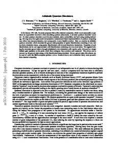
problem. In the circuit model of quantum computation, the oracle takes the form of a unitary matrix that flips the sign of the phase of each basis state that corresponds to a solution. This oracle can be constructed as a permutative circuit that inverts an ancilla qubit for every solution state. Initializing the ancilla qubit to the state √12 |0i − √12 |1i then results in a unitary operator that will flip the sign of the desired basis states due to phase kick-back. The adiabatic quantum version of Grover’s algorithm takes the form of a Hamiltonian in which the solution states correspond to low energy levels. This oracle Hamiltonian can then be used to construct a Hamiltonian that will evolve to one of the solution states. Because the oracle is necessary for Grover’s algorithm, implementing the Hamiltonian for the oracle is an important problem. Biamonte [2] developed a method for mapping a binary circuit represented as a planar tree of two-input single-output gates into 3-local Hamiltonians. This method is illustrated by mapping the tree of gates shown in figure 1(a) onto the two-dimensional grid of qubits shown in figure 1(b). The operation I used in nodes with exactly one input indicates that the value of the node is copied from the input. In this paper, the grid utilized in D-Wave’s prototype is used where each node has eight neighbors. These 3-local Hamiltonians are then decomposed into 2-local Hamiltonians which allows the desired circuit to be implemented on an adiabatic quantum computer. The main problem with this method [2] is that it is not algorithmic and no proof is provided that it is always even possible to map the tree of gates to the two-dimensional grid of qubits. Furthermore, no evidence is provided that this can be done efficiently. Backtracking is also required when this method is used because it is possible to reach a partial solution from which the final solution cannot be reached. This will cause any algorithm that uses this method to run slowly for large problems without the use of sophisticated heuristics. In this paper, a mapping method is shown which is capable of mapping a binary function to the two-dimensional grid of qubits while avoiding the difficulties with layout that result from using the method proposed by Biamonte [2]. Furthermore, the method shown in this paper is completely algorithmic and also does not require backtracking. Mapping is performed by first writing the desired binary function in a special form which can be implemented efficiently by decomposing it to the Hamiltonians given by Biamonte [2].

2

Introduction to Adiabatic Quantum Computation

This section will cover the basic principles of adiabatic quantum computation and will present some of the Hamiltonians developed by Biamonte [2]. Rather than applying operations to an input state as in the circuit model of quantum computation, the adiabatic model of quantum computation is based on the evolution of Hamiltonians. A Hamiltonian is a hermitian matrix that represents the energy of a quantum system. The eigenvalues of a Hamiltonian correspond to the energies of the eigenvectors. The state |ψ(t)i of a quantum system with the

2

Hamiltonian H(t) at time t and initial state |ψ(0)i is governed by Schr¨odinger’s equation [5] d |ψ(t)i = H(t) |ψ(t)i (1) i~ dt The Hamiltonians given by Biamonte [2] will now be presented. Let σ be the 2 × 2 hermitian matrix such that σ |0i = |0i and σ |1i = − |1i. Let σi = I2i−1 ⊗σ ⊗I2n−i where n is the number of qubits. Qubits can be initialized using the Hamiltonian I2n2−σi to set the ith qubit to |0i and the Hamiltonian I2n2+σi to set the ith qubit to |1i. This is because during adiabatic quantum computation the state of the system evolves to a minimal energy state. Since the eigenvectors of the Hamiltonian I2n2−σi are |x1 . . . xi−1 0xi+1 . . . xn i with eigenvalue 0 and |x1 . . . xi−1 1xi+1 . . . xn i with eigenvalue 1, using this Hamiltonian will cause the state of the ith qubit to evolve to |0i. Similar reasoning can be employed to explain why the Hamiltonian I2n2+σi initializes the ith qubit to |1i. Another I n −σ σ useful Hamiltonian is 2 2 i j which causes the ith and j th qubits to evolve to the same value. This works because σi |x1 . . . xn i = (−1)xi |x1 . . . xn i so xi +xj +1 1+(−1)xi +xj +1 |x1 . . . xn i. Since 1+(−1)2 |x1 . . . xn i = 2 1+(−1)xi +xj +1 0 · |x1 . . . xn i if xi = xj and |x1 . . . xn i = |x1 . . . xn i if xi 6= xj , the 2 energy of any basis state |x1 . . . xn i is 0 if xi = xj and is 1 if xi 6= xj . Biamonte

I2n −σi σj 2

|x1 . . . xn i =

also showed how to realize any two-input single-output gate using two-local Hamiltonians [2] except exclusive OR (EXOR) and its negation (EQUIV) which can be implemented with 2-local Hamiltonians by adding additional qubits. 6

x1

5

x2

4

x3

3

x4

∧

2

x5

∧

1

x6

x1 x 2 x3 x 4 x5 x 6

1

(a) An example tree of gates

∧ I

2

∨

∨

3

4

(b) A possible grid of qubits

Figure 1: An example of Biamonte’s method for mapping trees of gates to two-dimensional grids of qubits

3

3

A Generalized Sum of Products

A sum of products (SOP) is a simple formula that can be used to express any binary function. This is done by writing a binary function s of the variables x1 , . . . , xn as m _ s(x1 , . . . , xn ) = pi (2) i=1

where pi =

n ^

vi,j

(3)

j=1

Each vi,j must be in the set {1, xj , xj } and m is the number of products in the SOP. Using the method shown by Biamonte [2], it is possible to implement all 16 binary gates with two inputs and a single output using 3-local Hamiltonians. All of these 3-local Hamiltonians can be written as sums of 2-local Hamiltonians except for the 3-local Hamiltonians used for EXOR and EQUIV. This allows all of these gates to be implemented directly except for EXOR and EQUIV which must be decomposed to gates in the NPN classification of AND. Thus, all gates except EXOR and EQUIV are of the same cost. This means that a more general summation formula should be used because this will allow some functions to be implemented using far fewer products which will result in smaller number of qubits used. Since most of the operations in a SOP occur inside products, these operations should have small costs. However, the number of operations used to sum the products is comparatively small so even if these operations are fairly expensive, it will not significantly increase the overall cost of the circuit. The concept of a SOP was therefore generalized to represent a binary function s of the variables x1 , . . . , xn as s = sm where s1 = p1

(4)

si = gi−1 (pi , si−1 ) for 1 < i ≤ m

(5)

pi = pi,n

(6)

pi,1 = x1

(7)

pi,j = fi,j−1 (xj , pi,j−1 ) for 1 < j ≤ n

(8)

For these equations, the conditions m ≥ 1 and n ≥ 2 must hold. The conditions fi,j ∈ F and gi ∈ G must be satisfied where G = {g : {0, 1}2 → {0, 1}}, F = G\{⊕, } and the symbols ⊕ and represent EXOR and EQUIV respectively. The idea is to create a generalized sum of generalized products where each generalized product is created using any two-input single-output gates except for EXOR and EQUIV and the generalized sum can be created using any twoinput single-output gates. Since the set of all two-input binary gates except for EXOR and EQUIV is the NPN class of AND (the set of all gates that can be obtained by negating and permuting inputs and negating the output of an AND gate), the formula defined by equations (4) and (5) will be called an 4

NPNSOP. Note that functions in product of sums (POS) are included in the NPNSOP form. Since the summing operations do not all have to be the same function, the order in which the summing operations are applied affects the function that the NPNSOP represents. This is different from a SOP in which all of the summing operations are the OR operation. Note that the NPNSOP defines the order in which the summing operations are applied explicitly. This will simplify mapping to the grid of qubits later on and is the main reason why prefix notation is used. The generalized products (these will be called NPN products from now on) are represented by equations (7) and (8). Note that the order in which the product operations are applied is also defined explicitly which is important since the operations in a NPN product can be different functions. An example of a function represented by s = sm as defined by equations (4) through (8) will be shown later in this paper.

4

A Simple Example

This section will illustrate the mapping algorithm for the function s = ∨ (∧(x4 , I1 (x3 , z(x2 , x1 ))),

(9)

⊕ (∨(x4 , I2 (x3 , ∧(x2 , x1 ))), I2 (x4 , ∧(x3 , I1 (x2 , x1 ))))) written in pure NPNSOP form as defined by equations equations (4) through (8) where I1 (x, y) = x, I2 (x, y) = y and z(x, y) = 0. Using infix notation, this function can be written as s = x4 ∧ x3 ∨ ((x4 ∨ x2 ∧ x1 ) ⊕ x3 ∧ x2 )

(10)

In boolean algebra the function would be written as s = x4 x3 + ((x4 + x2 x1 ) ⊕ x3 x2 )

(11)

The function s can be visualized using a Karnaugh map as shown in figure 2. This function can be implemented using the grid of qubits shown in figure 3. The symbols that each node is labeled with indicate the binary operation that corresponds to the given node and the arrows indicate that the values of nodes that the arrows come from are arguments to the binary operation pointed to by the arrows. Solid arrows indicate that the value is not negated while dashed arrows indicate negation. For example, the function realized by the node at coordinates (8, 3) (the node in column 8 and row 3) is ∧(x4 , x3 ).

5

The Mapping Algorithm

An algorithm for mapping functions represented using the NPNSOP form defined by equations (4) through (8) will now be shown. The idea is to realize each

5

x3 s

x4 1 0

1 1

1 x2

2

10

0 15

1 9

1 6

1

1 8

0 7

11

0 4

1 3

1 x1

1 5

0 14

1 13

0 12

Figure 2: The Karnaugh map for the function s as defined in equation (9)

6

x1

5

x2

2 1

x1 x2

I1

4

x3

3

2 x4 1 I2

x3

∧

x1 x2

∧ 2 1 I2

0

2 x3 1 I1

x4

∨

x4 I

∧

2

I

I

∧

1

I

I

∧

∨

I

∨

3

4

5

6

7

8

s

1

2

9

Figure 3: The grid of qubits for the function s from equation 9

6

of the NPN products pi and “add” them into the NPNSOP. This is accomplished using the pseudocode shown in algorithm 1. The qubits used in the algorithm are mapped to a two dimensional grid as shown in figure 3 where the qubit with coordinates (x, y) is denoted by ax,y . The notation x1 , . . . , xn → ak,n+2 , . . . , ak,3 used on line 5 indicates that each of the qubits ak,n+2 , . . . , ak,3 is initialized to one of the values x1 , . . . , xn respectively. Several other conventions are used to describe the operation of the algorithm. The notation ax1 ,y1 →I ax2 ,y2 indicates that a Hamiltonian should be created that has the lowest energy when the qubits ax1 ,y1 and ax2 ,y2 have the same value. This Hamiltonian can be created as described by Biamonte [2]. Let h be a binary function of two variables. Then the notation ax1 ,y1 , ax2 ,y2 →h ax3 ,y3 indicates that a Hamiltonian should be created where the lowest energy state occurs when ax3 ,y3 = h(ax1 ,y1 , ax2 ,y2 ). Sometimes, the function h is written as a binary formula using the variables x and y. In this case, x corresponds to the first argument of h and y corresponds to the second argument of h. These Hamiltonians can be implemented using the method described by Biamonte [2]. Note that algorithm 1 uses more columns than necessary in some case such as column 3 in figure 3. This is done because it makes the algorithm much simpler and only affects the number of qubits it uses by a constant factor. Furthermore, in a practical application it would be simple to remove wasted columns by running an additional compaction algorithm to optimize the output of algorithm 1. Algorithm 1 also uses more operations than necessary to implement NPN products in some cases. This is also done for simplicity and would be easily rectified in an implementation of the algorithm. Algorithm 1 works by synthesizing each NPN product and then combining it into the NPNSOP. This is done by the loop on lines 3 to 29 which iterates over all m NPN products. During each iteration, the NPN product pi is mapped on the grid of qubits. Line 4 sets k to the index of the column where the values of the input variables for the NPN product pi . Line 5 stores the values of the inputs variables in the column with index k. The code on line 6 stores the value fi,1 (x2 , x1 ) in the qubit ak+1,n+1 . The rest of the NPN product pi is then mapped to the grid of qubits by the loop on lines 7 to 9. At this point in the algorithm, pi is stored in the qubit ak+1,3 . The rest of the code deals with “adding” pi into the NPNSOP. Line 10 tests if i = 1. If this is the case than pi is the first NPN product in the NPNSOP so it does not need to be “added” into the NPNSOP of previous NPN products so the value of pi is simply copied into the qubit ak+2,1 . This is done because during all iterations after the first iteration the value si−1 as defined in equations (4) and (5) is assumed to be stored in the qubit ak−1,1 . Lines 13 to 28 deal with the case where i 6= 1. In this case, si−1 is stored in the qubit ak−1,1 . Line 14 copies pi into the qubit ak,2 . Line 15 copies si−1 into the qubit ak,1 . Because the operations EXOR and EQUIV cannot be implemented using a single operation [2], it is necessary to implement them using the identities x ⊕ y = xy + xy and x y = xy + xy. The case where gi−1 = ⊕ or gi−1 = therefore must be handled separately. Line 16 accomplishes this by checking if gi−1 is neither EXOR nor EQUIV. If this is the case then gi−1 is mapped to the grid of qubits directly on line 17. Line 18 copies the result from the qubit ak+1,1 to the qubit ak+2,1 so that the 7

partial NPNSOP will be in the location expected by the next iteration of the outer loop. Line 19 handles the other case where gi−1 = ⊕ or gi−1 = . In this case, line 20 stores pi si−1 in the qubit ak+1,2 and line 21 stores pi si−1 in the qubit ak+1,1 . Line 23 checks if gi−1 = ⊕. If this is the case then the EXOR operation is performed by storing the OR of the qubits ak+1,1 and ak+1,2 in the qubit ak+2,1 on line 23. Otherwise, gi−1 = . This case is handled by line 25 which stores the NOR of the qubits ak+1,1 and ak+1,2 in the qubit ak+2,1 . Algorithm 1 Pseudocode for the mapping algorithm 1: Let s be a binary function in NPNSOP form as defined in equations (4) through (8) 2: Let m, n, fi,j , gi be as defined in equations (4) through (8) with respect to s 3: for all i := 1, . . . , m do 4: k := 3(i − 1) + 1 5: x1 , . . . , xn → ak,n+2 , . . . , ak,3 6: ak,n+1 , ak,n+2 →fi,1 ak+1,n+1 7: for all j := 2, . . . , n − 1 do 8: ak,n−j+2 , ak+1,n−j+3 →fi,j ak+1,n−j+2 9: end for 10: if i = 1 then 11: a2,3 →I a3,2 12: a3,2 →I a3,1 13: else 14: ak+1,3 →I ak,2 15: ak−1,1 →I ak,1 16: if gi−1 6= ⊕ and gi−1 6= then 17: ak,2 , ak,1 →gi−1 ak+1,1 18: ak+1,1 →I ak+2,1 19: else 20: ak,2 , ak,1 →x∧y ak+1,2 21: ak,2 , ak,1 →x∧y ak+1,1 22: if gi−1 = ⊕ then 23: ak+1,2 , ak+1,1 →∨ ak+2,1 24: else 25: ak+1,2 , ak+1,1 →∨ ak+2,1 26: end if 27: end if 28: end if 29: end for

8

6

Correctness Proof for the Mapping Algorithm

This section will prove that algorithm 1 properly maps binary functions in NPNSOP form as defined by equations (4) through (8) to the grid of qubits. It will be assumed that the Hamiltonians given by Biamonte [2] work correctly. Theorem 6.1. Given a binary function s of the form defined by equations (4) through (8), algorithm 1 maps the output of the function s to the qubit a3m,1 . Proof. After line 1, s is a binary function in NPNSOP form as defined by equations (4) through (8). Line 2 sets the variables m, n, fi,j and gi according to the values they are assigned when s is defined according to equations (4) through (8). Let si be as defined by equations (4) and (5). To simplify to proof, the concept of an unused qubit will be introduced. A qubit is said to be unused if the corresponding node on the grid of qubits has no inputs, has no outputs and has not been initialized to any particular value. Before using induction on the loop on line 3, it is necessary to prove that if the qubits in columns k and k + 1 are unused after line 4 is executed, then after executing lines 5 through 9 the qubit ak+1,3 stores pi and the qubits ak,j 0 and ak+1,j 0 are unused where j 0 ≤ 2. Line 5 initializes the qubits ak,n+2 , . . . , ak,3 to the variables x1 , . . . , xn and line 6 sets the qubit ak+1,n+1 equal to fi,1 (x2 , x1 ). Suppose that n = 2. Then the loop on line 7 will not run since the condition 2 ≤ n − 1 is false. Furthermore, pi,n = fi,1 (x2 , x1 ) and pi = pi,n in this case so the qubit ak+1,3 stores pi . Suppose that n > 2. In this case it is necessary to prove by induction that after each iteration of the loop on line 7, the qubit a2,n−j+2 stores pi,j and each qubit ak+1,j 0 where j 0 < n − j + 2 is unused. Consider the basis case where j = 2. Line 8 will perform the operation ak,n , ak+1,n+1 →fi,2 ak+1,n . Since the qubit ak,n stores x3 and the qubit ak+1,n+1 stores pi,1 = fi,1 (x2 , x1 ), this will result in the qubit ak+1,n storing pi,2 = fi,2 (x3 , pi,1 ). Furthermore, in column k + 1 the only qubits used are ak+1,n+1 and ak+1,n so the basis case holds. Now suppose that after the iteration where j = ˆj in the loop on line 7 the qubit ak+1,n−ˆj+2 stores pi,ˆj and that each qubit ak+1,j 0 where j 0 < n − ˆj + 2 is unused. Then at the start of the iteration where j = ˆj + 1, the qubit ak+1,n−ˆj+2 still stores pi,ˆj . Line 8 will perform the operation ak,n−ˆj+1 , ak+1,n−ˆj+2 →fi,ˆj+1 ak+1,n−ˆj+1 . Since the qubit ak+1,n−ˆj+1 stores xˆj+2 , the result of this operation is storing pi,ˆj+1 = fi,ˆj+1 (xˆj+2 , pi,ˆj ) in the qubit ak+1,n−ˆj+1 . Since each qubit ak+1,j 0 where j 0 < n − ˆj + 2 was unused before this operation was performed, each qubit ak+1,j 0 where j 0 < n − ˆj + 1 is unused afterward. This proves the inductive case so by the principle of mathematical induction, after the final iteration of the loop on line 7 the qubit ak+1,3 stores pi = pi,n and the qubits ak+1,2 and ak+1,1 are unused. It will now be proved by induction on i that after each iteration of the loop on line 3 the following hold: • The qubit ak+2,1 stores si • Each qubit ai0 ,j 0 is unused for i0 > k + 2

9

For the basis case, i = 1 so after line 4 is executed k = 1. Since all of the qubits are unused at this point, in particular the qubits in columns k and k + 1 are unused. Therefore, by the reasoning shown above, after executing lines 5 through 9 the qubit a2,3 stores pi and the qubits a1,j 0 and a2,j 0 are unused where j 0 ≤ 2. In particular, the qubits a2,2 and a2,1 are unused. Since i = 1, the if statement on line 10 causes lines 11 and 12 to be executed. Running line 11 causes s1 to be copied from the qubit a2,3 into the qubit a3,2 will store s1 . After executing line 12, s1 is copied into the qubit a3,1 . Since only qubits in the columns 1, 2 and 3 were used, this proves the basis case. The inductive case will now be considered. Assume that after the iteration of the loop on line 3 where i = ˆi that the qubit ak+2,1 stores sˆi each qubit ai0 ,j 0 is unused for i0 > kˆ + 2 ˆ where kˆ = 3(ˆi − 1) + 1 is the value of k in the ˆith iteration. Now consider the iteration of the loop where i = ˆi + 1. After executing line 4, k = 3(i − 1) + 1. As shown before, executing lines 5 through 9 causes the qubit ak+1,3 to store pˆi+1 and the qubits ak,j 0 and ak+1,j 0 to be unused where j 0 ≤ 2. Since i = ˆi + 1 and ˆi ≥ 1, i > 1. Therefore, executing the if statement on line 10 will cause lines 13 through 28 to be executed. Line 14 copies pˆi+1 into the qubit ak,2 . Observe that kˆ + 2 = k − 1. Therefore, line 15 copies sˆi into the qubit ak,1 . Suppose that gˆi 6= ⊕gˆi = . Then the if statement on line 16 will cause lines 17 through 18 to be executed. Executing line 17 will store sˆi+1 = gˆi (pˆi+1 , sˆi ) in the qubit ak+1,1 and line 18 will copy aˆi+1 into the qubit ak+2,1 . Now assume that the condition gˆi 6= ⊕gˆi = is false. In this case lines 19 through 27 will be executed. Line 20 stores p+1 ˆ sˆi in ˆ sˆi in the qubit ak+1,2 . Line 21 stores p+1 the qubit ak+1,1 . Because gˆi 6= ⊕gˆi = is false, gˆi = ⊕ or gˆi = . Suppose that gˆi = ⊕. Then the if statement on line 22 will cause line 23 to run which will result in p+1 ˆ ⊕ sˆi = p+1 ˆ sˆi + p+1 ˆ sˆi being stored the qubit ak+2,1 . Since gˆi = ⊕ and s+1 ˆ = p+1 ˆ ⊕ sˆi p+1 ˆ , sˆi+1 is stored in the qubit ak+2,1 . Now assume that gˆi = . In this case, the if statement on line 22 will cause line 25 to run. This will result in storing p+1 ˆ sˆi = p+1 ˆ sˆi + p+1 ˆ sˆi in the qubit ak+2,1 . Because sˆi+1 = p+1 ˆ sˆi in this case, sˆi+1 is stored in the qubit ak+2,1 . Thus, after the iteration of the loop on line 3 where i = ˆi + 1, sˆi+1 is stored in the qubit ak+2,1 . Because only qubits in the columns k, k + 1 and k + 2 were used in the iteration where i = ˆi + 1, each qubit ai0 ,j 0 is unused for i0 > k + 2 after this iteration is finished. Thus, the inductive case holds as well. Therefore, by the principle of mathematical induction, the following conditions hold after every iteration of the loop on line 3: • The qubit ak+2,1 stores si • Each qubit ai0 ,j 0 is unused for i0 > k + 2 Consequently, since i = m and k = (3m − 1) + 1 in the last iteration of the loop on line 3, the qubit a3m,1 stores s = sn after the loop finishes executing.

10

7

Complexity of the Algorithm

In this section, the complexity of algorithm 1 will be analyzed. This will be calculated in terms of the number of qubits required and the running time required by algorithm 1. Lines 1 and 2 do not use any qubits. Consequently, the total maximum number of required qubits can be calculated by determining the number of qubits used in each iteration of the loop. Each iteration of the loop on line 3 uses at least n qubits because of line 5. Also, since during each iteration only qubits ai0 ,j 0 with indexes satisfying k ≤ i0 ≤ k + 2 and 1 ≤ j 0 ≤ n + 2 can be used, each iteration requires at most 3(n + 2) qubits. Because the loop on line 3 is executed m times, between mn and 3m(n + 2) qubits are used by each iteration. Therefore, the number of qubits required is bounded above and below by positive multiples of mn so the number of qubits required is Θ(mn). The running time complexity of algorithm 1 will now be determined. Observe that all of the steps in the loop on lines 3 to 29 run in constant time except for the loop on lines 7 to 9 which requires n − 2 operations. This implies that each iteration of the loop requires Θ(n) operations so the entire loop uses Θ(mn) operations.

8

Advantages of the Algorithm

Algorithm 1 has some important advantages over the mapping method proposed by Biamonte [2]. Algorithm 1 is totally algorithmic and does not require trees of gates to be mapped onto the two dimensional grid of qubits which is required if the Biamonte’s mapping method [2] is used. This resolves a significant problem with the Biamonte method [2] because it eliminates the necessity of using long chains of qubits to repeat values of qubits. Algorithm 1 does not have this problem because it only performs operations on adjacent qubits. Algorithm 1 is also reasonably efficient as it requires Θ(mn) qubits.

9

Conclusion

This paper presented a mapping algorithm for adiabatic quantum computation which is more practical than previous methods because it does not waste large amounts of qubits repeating intermediate values. The algorithm is capable of synthesizing a very general class of boolean formulas and is also fairly efficient since it uses only Θ(mn) qubits. This makes this algorithm a good method for synthesizing oracles for the adiabatic quantum version of Grover’s algorithm [6].

References [1] D. Aharonov, W. van Dam, J. Kempe, Z. Landau, S. Lloyd, and O. Regev. Adiabatic quantum computation is equivalent to standard quantum computation. arXiv:quant-ph/0405098v2, 2005.

11

[2] J. D. Biamonte. Non-perturbative k-body to two-body commuting conversion hamiltonians and embedding problem instances into ising spins. Physical Review A, 77:23–31, 2008. [3] L. K. Grover. A fast quantum mechanical algorithm for database search. In Proceedings of the Annual ACM Symposium on Theory of Computing, pages 212–219, 1996. [4] R. Harris, F. Brito, A. J. Berkely, J. Johansson, M. W. Johnson, T. Lanting, P. Bunyk, E. Ladizinsky, B. Bumble, A. Fung, A. Kaul, A. Kleinsasser, and S. Han. Synchronization of multiple coupled rf-squid flux qubits. arXiv:0903.1884v1, 2009. [5] M. A. Nielsen and I. L. Chuang. Quantum Computation and Quantum Information. Cambridge University Press, 2000. [6] W. van Dam, M. Mosca, and U. Vazirani. How powerful is adiabatic quantum computation? arXiv:quant-ph/0206003v1, 2002.

12