MapReduce Based Parallel Neural Networks in Enabling Large Scale ...

Hindawi Publishing Corporation Computational Intelligence and Neuroscience Volume 2015, Article ID 297672, 13 pages http://dx.doi.org/10.1155/2015/297672

Research Article MapReduce Based Parallel Neural Networks in Enabling Large Scale Machine Learning Yang Liu,1 Jie Yang,1 Yuan Huang,1 Lixiong Xu,1 Siguang Li,2 and Man Qi3 1

School of Electrical Engineering and Information, Sichuan University, Chengdu 610065, China The Key Laboratory of Embedded Systems and Service Computing, Tongji University, Shanghai 200092, China 3 Department of Computing, Canterbury Christ Church University, Canterbury, Kent CT1 1QU, UK 2

Correspondence should be addressed to Lixiong Xu; [email protected] Received 28 May 2015; Accepted 11 August 2015 Academic Editor: Ladislav Hluchy Copyright © 2015 Yang Liu et al. This is an open access article distributed under the Creative Commons Attribution License, which permits unrestricted use, distribution, and reproduction in any medium, provided the original work is properly cited. Artificial neural networks (ANNs) have been widely used in pattern recognition and classification applications. However, ANNs are notably slow in computation especially when the size of data is large. Nowadays, big data has received a momentum from both industry and academia. To fulfill the potentials of ANNs for big data applications, the computation process must be speeded up. For this purpose, this paper parallelizes neural networks based on MapReduce, which has become a major computing model to facilitate data intensive applications. Three data intensive scenarios are considered in the parallelization process in terms of the volume of classification data, the size of the training data, and the number of neurons in the neural network. The performance of the parallelized neural networks is evaluated in an experimental MapReduce computer cluster from the aspects of accuracy in classification and efficiency in computation.

1. Introduction Recently, big data has received a momentum from both industry and academia. Many organizations are continuously collecting massive amounts of datasets from various sources such as the World Wide Web, sensor networks, and social networks. In [1], big data is defined as a term that encompasses the use of techniques to capture, process, analyze, and visualize potentially large datasets in a reasonable time frame not accessible to standard IT technologies. Basically, big data is characterized with three Vs [2]: (i) Volume: the sheer amount of data generated. (ii) Velocity: the rate at which the data is being generated. (iii) Variety: the heterogeneity of data sources. Artificial neural networks (ANNs) have been widely used in pattern recognition and classification applications. Back-propagation neural network (BPNN), the most popular one of ANNs, could approximate any continuous nonlinear functions by arbitrary precision with an enough number of

neurons [3]. Normally, BPNN employs the back-propagation algorithm for training which requires a significant amount of time when the size of the training data is large [4]. To fulfill the potentials of neural networks in big data applications, the computation process must be speeded up with parallel computing techniques such as the Message Passing Interface (MPI) [5, 6]. In [7], Long and Gupta presented a scalable parallel artificial neural network using MPI for parallelization. It is worth noting that MPI was designed for data intensive applications with high performance requirements. MPI provides little support in fault tolerance. If any fault happens, an MPI computation has to be started from the beginning. As a result, MPI is not suitable for big data applications, which would normally run for many hours during which some faults might happen. This paper presents a MapReduce based parallel backpropagation neural network (MRBPNN). MapReduce has become a de facto standard computing model in support of big data applications [8, 9]. MapReduce provides a reliable, fault-tolerant, scalable, and resilient computing framework for storing and processing massive datasets. MapReduce

2 scales well with ever increasing sizes of datasets due to its use of hash keys for data processing and the strategy of moving computation to the closest data nodes. In MapReduce, there are mainly two functions which are the Map function (mapper) and the Reduce function (reducer). Basically, a mapper is responsible for actual data processing and generates intermediate results in the form of ⟨key, value⟩ pairs. A reducer collects the output results from multiple mappers with secondary processing including sorting and merging the intermediate results based on the key values. Finally the Reduce function generates the computation results. We present three MRBPNNs (i.e., MRBPNN 1, MRBPNN 2, and MRBPNN 3) to deal with different data intensive scenarios. MRBPNN 1 deals with a scenario in which the dataset to be classified is large. The input dataset is segmented into a number of data chunks which are processed by mappers in parallel. In this scenario, each mapper builds the same BPNN classifier using the same set of training data. MRBPNN 2 focuses on a scenario in which the volume of the training data is large. In this case, the training data is segmented into data chunks which are processed by mappers in parallel. Each mapper still builds the same BPNN but uses only a portion of the training dataset to train the BPNN. To maintain a high accuracy in classification, we employ a bagging based ensemble technique [10] in MRBPNN 2. MRBPNN 3 targets a scenario in which the number of neurons in a BPNN is large. In this case, MRBPNN 3 fully parallelizes and distributes the BPNN among the mappers in such a way that each mapper employs a portion of the neurons for training. The rest of the paper is organized as follows. Section 2 gives a review on the related work. Section 3 presents the designs and implementations of the three parallel BPNNs using the MapReduce model. Section 4 evaluates the performance of the parallel BPNNs and analyzes the experimental results. Section 5 concludes the paper.

2. Related Work ANNs have been widely applied in various pattern recognition and classification applications. For example, Jiang et al. [11] employed a back-propagation neural network to classify high resolution remote sensing images to recognize roads and roofs in the images. Khoa et al. [12] proposed a method to forecast the stock price using BPNN. Traditionally, ANNs are employed to deal with a small volume of data. With the emergence of big data, ANNs have become computationally intensive for data intensive applications which limits their wide applications. Rizwan et al. [13] employed a neural network on global solar energy estimation. They considered the research as a big task, as traditional approaches are based on extreme simplicity of the parameterizations. A neural network was designed which contains a large number of neurons and layers for complex function approximation and data processing. The authors reported that in this case the training time will be severely affected. Wang et al. [14] pointed out that currently large scale neural networks are one of the mainstream tools for big data analytics. The challenge in processing big data with large scale

Computational Intelligence and Neuroscience neural networks includes two phases which are the training phase and the operation phase. To speed up the computations of neural networks, there are some efforts that try to improve the selection of initial weights [15] or control the learning parameters [16] of neural networks. Recently, researchers have started utilizing parallel and distributed computing technologies such as cloud computing to solve the computation bottleneck of a large neural network [17–19]. Yuan and Yu [20] employed cloud computing mainly for exchange of privacy data in a BPNN implementation in processing ciphered text classification tasks. However, cloud computing as a computing paradigm simply offers infrastructure as a service (IaaS), platform as a service (PaaS), and software as a service (SaaS). It is worth noting that cloud computing still needs big data processing models such as the MapReduce model to deal with data intensive applications. Gu et al. [4] presented a parallel neural network using in-memory data processing techniques to speed up the computation of the neural network but without considering the accuracy aspect of the implemented parallel neural network. In this work, the training data is simply segmented into data chunks which are processed in parallel. Liu et al. [21] presented a MapReduce based parallel BPNN in processing a large set of mobile data. This work further employs AdaBoosting to accommodate the loss of accuracy of the parallelized neural network. However, the computationally intensive issue may exist not only at the training phase but also at the classification phase. In addition, AdaBoosting is a popular sampling technique; it may enlarge the weights of wrongly classified instances which would deteriorate the algorithm accuracy.

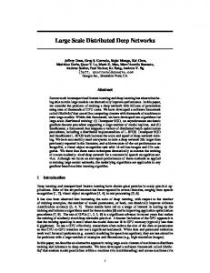
3. Parallelizing Neural Networks This section presents the design details of the parallelized MRBPNN 1, MRBPNN 2, and MRBPNN 3. First, a brief review of BPNN is introduced. 3.1. Back-Propagation Neural Network. Back-propagation neural network is a multilayer feed forward network which trains the training data using an error back-propagation mechanism. It has become one of the most widely used neural networks. BPNN can perform a large volume of input-output mappings without knowing their exact mathematical equations. This benefits from the gradient-descent feature of its back-propagation mechanism. During the error propagation, BPNN keeps tuning the parameters of the network until it adapts to all input instances. A typical BPNN is shown in Figure 1, which consists of an arbitrary number of inputs and outputs. Generally speaking, a BPNN can have multiple network layers. However, it has been widely accepted that a three-layer BPNN would be enough to fit the mathematical equations which approximate the mapping relationships between inputs and outputs [3]. Therefore, the topology of a BPNN usually contains three layers: input layer, one hidden layer, and output layer. The number of inputs in the input layer is mainly determined by the number of elements in an input eigenvector; for instance, let s denote an input instance: s = {𝑎1 , 𝑎2 , 𝑎3 , . . . , 𝑎𝑛 } .

(1)

Computational Intelligence and Neuroscience

3

x0

∫

∫

∫

y0

x1

∫

∫

∫

y1

.. .

.. .

.. .

∫

∫

∫

.. . xn−1

The input keeps training the network until (7) is satisfied for a single output or (8) is satisfied for multiple outputs: min (𝐸 [𝑒2 ]) = min (𝐸 [(𝑡 − 𝑜)2 ]) , min (𝐸 [𝑒𝑇 𝑒]) = min (𝐸 [(𝑡 − 𝑜)𝑇 (𝑡 − 𝑜)]) .

yn−1

Figure 1: The structure of a typical BPNN.

Then, the number of inputs is 𝑛. Similarly, the number of neurons in the output layer is determined by the number of classifications. And the number of neurons in the hidden layer is determined by users. Every input of a neuron has a weight 𝑤𝑖𝑗 , where 𝑖 and 𝑗 represent the source and destination of the input. Each neuron also maintains an optional parameter 𝜃𝑗 which is actually a bias for varying the activity of the 𝑗th neuron in a layer. Therefore, let 𝑜𝑗󸀠 denote the output from a previous neuron and let 𝑜𝑗 denote the output of this layer; the input 𝐼𝑗 of neurons located in both the hidden and output layer can be represented by 𝐼𝑗 = ∑𝑤𝑖𝑗 𝑜𝑗󸀠 + 𝜃𝑗 . 𝑖

(2)

The output of a neuron is usually computed by the sigmoid function, so the output 𝑜𝑗 can be computed by 1 𝑜𝑗 = . 1 + 𝑒−𝐼𝑗

(3)

After the feed forward process is completed, the backpropagation process starts. Let Err𝑗 represent the errorsensitivity and let 𝑡𝑗 represent the desirable output of neuron 𝑗 in the output layer; thus, Err𝑗 = 𝑜𝑗 (1 − 𝑜𝑗 ) (𝑡𝑗 − 𝑜𝑗 ) .

(4)

Let Err𝑘 represent the error-sensitivity of one neuron in the last layer and let 𝑤𝑘𝑗 represent its weight; thus, Err𝑗 of a neuron in the other layers can be computed using Err𝑗 = 𝑜𝑗 (1 − 𝑜𝑗 ) ∑Err𝑘 𝑤𝑘𝑗 .

(7) (8)

3.2. MapReduce Computing Model. MapReduce has become the de facto standard computing model in dealing with data intensive applications using a cluster of commodity computers. Popular implementations of the MapReduce computing model include Mars [22], Phoenix [23], and Hadoop framework [24, 25]. The Hadoop framework has been widely taken up by the community due to its open source feature. Hadoop has its Hadoop Distributed File System (HDFS) for data management. A Hadoop cluster has one name node (Namenode) and a number of data nodes (Datanodes) for running jobs. The name node manages the metadata of the cluster whilst a data node is the actual processing node. The Map functions (mappers) and Reduce functions (reducers) run on the data nodes. When a job is submitted to a Hadoop cluster, the input data is divided into small chunks of an equal size and saved in the HDFS. In terms of data integrity, each data chunk can have one or more replicas according to the cluster configuration. In a Hadoop cluster, mappers copy and read data from either remote or local nodes based on data locality. The final output results will be sorted, merged, and generated by reducers in HDFS. 3.3. The Design of MRBPNN 1. MRBPNN 1 targets the scenario in which BPNN has a large volume of testing data to be classified. Consider a testing instance 𝑠𝑖 = {𝑎1 , 𝑎2 , 𝑎3 , . . . , 𝑎𝑖𝑛 }, 𝑠𝑖 ∈ 𝑆, where (i) 𝑠𝑖 denotes an instance; (ii) 𝑆 denotes a dataset; (iii) 𝑖𝑛 denotes the length of 𝑠𝑖 ; it also determines the number of inputs of a neural network; (iv) the inputs are capsulated ⟨instance𝑘 , target𝑘 , type⟩;

by

a

format

of

(v) instance𝑘 represents 𝑠𝑖 , which is the input of a neural network;

(5)

(vi) target𝑘 represents the desirable output if instance𝑘 is a training instance;

After Err𝑗 is computed, the weights and biases of each neuron are tuned in back-propagation process using

(vii) type field has two values, “train” and “test,” which marks the type of instance𝑘 ; if “test” value is set, target𝑘 field should be left empty.

𝑘

Δ𝑤𝑖𝑗 = Err𝑗 𝑜𝑗 , 𝑤𝑖𝑗 = 𝑤𝑖𝑗 + Δ𝑤𝑖𝑗 , Δ𝜃𝑗 = Err𝑗 ,

(6)

𝜃𝑗 = 𝜃𝑗 + Δ𝜃𝑗 . After the first input vector finishes tuning the network, the next round starts for the following input vectors.

Files which contain instances are saved into HDFS initially. Each file contains all the training instances and a portion of the testing instances. Therefore, the file number 𝑛 determines the number of mappers to be used. The file content is the input of MRBPNN 1. When the algorithm starts, each mapper initializes a neural network. As a result, there will be 𝑛 neural networks in the cluster. Moreover, all the neural networks have exactly the same structure and parameters. Each mapper reads data in

4

Computational Intelligence and Neuroscience a critical issue is that the classification accuracy of a mapper will be significantly degraded using only a portion of the training data. To solve this issue, MRBPNN 2 employs ensemble technique to maintain the classification accuracy by combining a number of weak learners to create a strong learner.

Data chunk 1 Training data

Mapper Data chunk 2

Training data

Mapper

.. .

Data chunk n

Training data

Mapper

Reducer

Final results

Figure 2: MRBPNN 1 architecture.

the form of ⟨instance𝑘 , target𝑘 , type⟩ from a file and parses the data records. If the value of type field is “train,” instance𝑘 is input into the input layer of the neural network. The network computes the output of each layer using (2) and (3), until the output layer generates an output which indicates the completion of the feed forward process. And then the neural network in each mapper starts the back-propagation process. It computes and updates new weights and biases for its neurons using (4) to (6). The neural network inputs instance𝑘+1 . Repeat the feed forward and back-propagation process until all the instances which are labeled as “train” are processed and the error is satisfied. Each mapper starts classifying instances labeled as “test” by running the feed forward process. As each mapper only classifies a portion of the entire testing dataset, the efficiency is improved. At last, each mapper outputs intermediate output in the form of ⟨instance𝑘 , 𝑜𝑗𝑚 ⟩, where instance𝑘 is the key and 𝑜𝑗𝑚 represents the output of the 𝑚th mapper. One reducer starts collecting and merging all the outputs of the mappers. Finally, the reducer outputs ⟨instance𝑘 , 𝑜𝑗𝑚 ⟩ into HDFS. In this case, 𝑜𝑗𝑚 represents the final classification result of instance𝑘 . Figure 2 shows the architecture of MRBPNN 1 and Algorithm 1 shows the pseudocode. 3.4. The Design of MRBPNN 2. MRBPNN 2 focuses on the scenario in which a BPNN has a large volume of training data. Consider a training dataset 𝑆 with a number of instances. As shown in Figure 3, MRBPNN 2 divides 𝑆 into 𝑛 data chunks of which each data chunk 𝑠𝑖 is processed by a mapper for training, respectively: 𝑛

𝑆 = ⋃ 𝑠𝑖 , 1

{∀𝑠 ∈ 𝑠𝑖 | 𝑠 ∉ 𝑠𝑛 , 𝑖 ≠ 𝑛} .

(9)

3.4.1. Bootstrapping. Training diverse classifiers from a single training dataset has been proven to be simple compared with the case of finding a strong learner [26]. A number of techniques exist for this purpose. A widely used technique is to resample the training dataset based on bootstrap aggregating such as bootstrapping and majority voting. This can reduce the variance of misclassification errors and hence increases the accuracy of the classifications. As mentioned in [26], balanced bootstrapping can reduce the variance when combining classifiers. Balanced bootstrapping ensures that each training instance equally appears in the bootstrap samples. It might not be always the case that each bootstrapping sample contains all the training instances. The most efficient way of creating balanced bootstrap samples is to construct a string of instances 𝑋1 , 𝑋2 , 𝑋3 , . . . , 𝑋𝑛 repeating 𝐵 times so that a sequence of 𝑌1 , 𝑌2 , 𝑌3 , . . . , 𝑌𝐵𝑛 can be achieved. A random permutation 𝑝 of the integers from 1 to 𝐵𝑛 is taken. Therefore, the first bootstrapping sample can be created from 𝑌𝑝 (1), 𝑌𝑝 (2), 𝑌𝑝 (3), . . . , 𝑌𝑝 (𝑛). In addition, the second bootstrapping sample is created from 𝑌𝑝 (𝑛+1), 𝑌𝑝 (𝑛+ 2), 𝑌𝑝 (𝑛 + 3), . . . , 𝑌𝑝 (2𝑛) and the process continues until 𝑌𝑝 ((𝐵−1)𝑛+1), 𝑌𝑝 ((𝐵−1)𝑛+2), 𝑌𝑝 ((𝐵−1)𝑛+3), . . . , 𝑌𝑝 (𝐵𝑛) is the 𝐵th bootstrapping sample. The bootstrapping samples can be used in bagging to increase the accuracy of classification. 3.4.2. Majority Voting. This type of ensemble classifiers performs classifications based on the majority votes of the base classifiers [26]. Let us define the prediction of the 𝑖th classifier 𝑃𝑖 as 𝑃𝑖,𝑗 ∈ {1, 0}, 𝑖 = 1, . . . , 𝐼 and 𝑗 = 1, . . . , 𝑐, where 𝐼 is the number of classifiers and 𝑐 is the number of classes. If the 𝑖th classifier chooses class 𝑗, then 𝑃𝑖,𝑗 = 1; otherwise, 𝑃𝑖,𝑗 = 0. Then, the ensemble prediction for class 𝑘 is computed using 𝑐

𝐼

𝑃𝑖,𝑘 = max∑𝑃𝑖,𝑗 . 𝑗=1

(11)

𝑖=1

3.4.3. Algorithm Design. At the beginning, MRBPNN 2 employs balanced bootstrapping to generate a number of subsets of the entire training dataset: balanced bootstrapping 󳨀→ {𝑆1 , 𝑆2 , 𝑆3 , . . . , 𝑆𝑛 } , 𝑛

Each mapper in the Hadoop cluster maintains a BPNN, and each 𝑠𝑖 is considered as the input training data for the neural network maintained in mapper𝑖 . As a result, each BPNN in a mapper produces a classifier based on the trained parameters:

⋃ 𝑆𝑖 = 𝑆,

(12)

𝑖=1

(10)

where 𝑆𝑖 represents the 𝑖th subset, which belongs to entire dataset 𝑆. 𝑛 represents the total number of subsets. Each 𝑆𝑖 is saved in one file in HDFS. Each instance 𝑠𝑘 = {𝑎1 , 𝑎2 , 𝑎3 , . . . , 𝑎𝑖𝑛 }, 𝑠𝑘 ∈ 𝑆𝑖 , is defined in the format of ⟨instance𝑘 , target𝑘 , type⟩, where

To reduce the computation overhead, each classifier𝑖 is trained with a part of the original training dataset. However,

(i) instance𝑘 represents one bootstrapped instance 𝑠𝑘 , which is the input of neural network;

(mapper𝑖 , BPNN𝑖 , 𝑠𝑖 ) 󳨀→ classifier𝑖 .

Computational Intelligence and Neuroscience

5

Sample 1

Data chunk MR 1

Sample 2

Data chunk

MR 2

Training data Sample 3 .. . Sample n

Data chunk MR 3 .. . Data chunk MR n

Reduce collects results of all BPNNs Major voting

Figure 3: MRBPNN 2 architecture.

Input: 𝑆, 𝑇 Output: 𝐶 𝑚 mappers one reducer (1) Each mapper constructs one BPNN with 𝑖𝑛 inputs, 𝑜 outputs, ℎ neurons in hidden layer (2) Initialize 𝑤𝑖𝑗 = random1𝑖𝑗 ∈ (−1, 1), 𝜃𝑗 = random2𝑗 ∈ (−1, 1) (3) ∀𝑠 ∈ 𝑆, 𝑠𝑖 = {𝑎1 , 𝑎2 , 𝑎3 , . . . , 𝑎𝑖𝑛 } Input 𝑎𝑖 → 𝑖𝑛𝑖 , neuron𝑗 in hidden layer computes 𝑖𝑛

𝐼𝑗ℎ = ∑ 𝑎𝑖 ⋅ 𝑤𝑖𝑗 + 𝜃𝑗 𝑖=1

1 1 + 𝑒𝐼𝑗ℎ (4) Input 𝑜𝑗 → out𝑖 , neuron𝑗 in output layer computes 𝑜𝑗ℎ =

ℎ

𝐼𝑗𝑜 = ∑ 𝑜𝑗ℎ ⋅ 𝑤𝑖𝑗 + 𝜃𝑗 𝑖=1

1 1 + 𝑒𝐼𝑗𝑜 (5) In each output, compute Err𝑗𝑜 = 𝑜𝑗𝑜 (1 − 𝑜𝑗𝑜 ) (target𝑗 − 𝑜𝑗𝑜 ) (6) In hidden layer, compute 𝑜𝑗𝑜 =

𝑜

Err𝑗ℎ = 𝑜𝑗ℎ (1 − 𝑜𝑗ℎ ) ∑ Err𝑖 𝑤𝑖𝑜 𝑖=1

(7) Update 𝑤𝑖𝑗 = 𝑤𝑖𝑗 + 𝜂 ⋅ Err𝑗 ⋅ 𝑜𝑗 𝜃𝑗 = 𝜃𝑗 + 𝜂 ⋅ Err𝑗 Repeat (3), (4), (5), (6), (7) Until 2 min (𝐸 [𝑒2 ]) = min (𝐸 [(target𝑗 − 𝑜𝑗𝑜 ) ]) Training terminates 𝑚 (8) Divide 𝑇 into {𝑇1 , 𝑇2 , 𝑇3 , . . . , 𝑇𝑚 }, ⋃𝑖=0 𝑇𝑖 = 𝑇 (9) Each mapper inputs 𝑡𝑗 = {𝑎1 , 𝑎2 , 𝑎3 , . . . , 𝑎𝑖𝑛 }, 𝑡𝑗 ∈ 𝑇𝑖 (10) Execute (3), (4) (11) Mapper outputs ⟨𝑡𝑗 , 𝑜𝑗 ⟩ (12) Reducer collects and merges all ⟨𝑡𝑗 , 𝑜𝑗 ⟩ Repeat (9), (10), (11), (12) Until 𝑇 is traversed. (13) Reducer outputs 𝐶 End Algorithm 1: MRBPNN 1.

6

Computational Intelligence and Neuroscience (ii) 𝑖𝑛 represents the number of inputs of the neural network;

(iv) target𝑛 represents the encoded desirable output of a training instance instance𝑛 ;

(iii) target𝑘 represents the desirable output if instance𝑘 is a training instance;

(v) the list of {𝑤𝑖𝑗2 , 𝜃𝑗2 , . . . , 𝑤𝑖𝑗𝑙−1 , 𝜃𝑗𝑙−1 } represents the weights and biases for next layers; it can be extended based on the layers of the network; for a standard three-layer neural network, this option becomes {𝑤𝑖𝑗𝑜 , 𝜃𝑗𝑜 }.

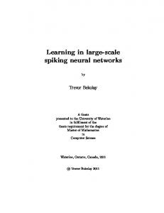
(iv) type field has two values, “train” and “test,” which marks the type of instance𝑘 ; if “test” value is set, target𝑘 field should be left empty. When MRBPNN 2 starts, each mapper constructs one BPNN and initializes weights and biases with random values between −1 and 1 for its neurons. And then a mapper inputs one record in the form of ⟨instance𝑘 , target𝑘 , type⟩ from the input file. The mapper firstly parses the data and retrieves the type of the instance. If the type value is “train,” the instance is fed into the input layer. Secondly, each neuron in different layers computes its output using (2) and (3) until the output layer generates an output which indicates the completion of the feed forward process. Each mapper starts a back-propagation process and computes and updates weights and biases for neurons using (4) to (6). The training process finishes until all the instances marked as “train” are processed and error is satisfied. All the mappers start feed forwarding to classify the testing dataset. In this case, each neural network in a mapper generates the classification result of an instance at the output layer. Each mapper generates an intermediate output in the form of ⟨instance𝑘 , 𝑜𝑗𝑚 ⟩, where instance𝑘 is the key and 𝑜𝑗𝑚 represents the outputs of the 𝑚th mapper. Finally, a reducer collects the outputs of all the mappers. The outputs with the same key are merged together. The reducer runs majority voting using (11) and outputs the result of instance𝑘 into HDFS in the form of ⟨instance𝑘 , 𝑟𝑘 ⟩, where 𝑟𝑘 represents the voted classification result of instance𝑘 . Figure 3 shows the algorithm architecture and Algorithm 2 presents the pseudocode of MRBPNN 2. 3.5. The Design of MRBPNN 3. MRBPNN 3 aims at the scenario in which a BPNN has a large number of neurons. The algorithm enables an entire MapReduce cluster to maintain one neural network across it. Therefore, each mapper holds one or several neurons. There are a number of iterations that exist in the algorithm with 𝑙 layers. MRBPNN 3 employs a number of 𝑙 − 1 MapReduce jobs to implement the iterations. The feed forward process runs in 𝑙 − 1 rounds whilst the back-propagation process occurs only in the last round. A data format in the form of ⟨index𝑘 , instance𝑛 , 𝑤𝑖𝑗 , 𝜃𝑗 , target𝑛 , {𝑤𝑖𝑗2 , 𝜃𝑗2 , . . . , 𝑤𝑖𝑗𝑙−1 , 𝜃𝑗𝑙−1 }⟩ has been designed to guarantee the data passing between Map and Reduce operations, where (i) index𝑘 represents the 𝑘th reducer; (ii) instance𝑛 represents the 𝑛th training or testing instance of the dataset; one instance is in the form of instance𝑛 = {𝑎1 , 𝑎2 , . . . , 𝑎𝑖𝑛 }, where 𝑖𝑛 is length of the instance; (iii) 𝑤𝑖𝑗 represents a set of weights of an input layer, whilst 𝜃𝑗 represents the biases of the neurons in the first hidden layer;

Before MRBPNN 3 starts, each instance and the information defined by data format are saved in one file in HDFS. The number of the layers is determined by the length of {𝑤𝑖𝑗2 , 𝜃𝑗2 . . . , 𝑤𝑖𝑗𝑙−1 , 𝜃𝑗𝑙−1 } field. The number of neurons in the next layer is determined by the number of files in the input folder. Generally, different from MRBPNN 1 and MRBPNN 2, MRBPNN 3 does not initialize an explicit neural network; instead, it maintains the network parameters based on the data defined in the data format. When MRBPNN 3 starts, each mapper initially inputs one record from HDFS. And then it computes the output of a neuron using (2) and (3). The output is generated by a mapper, which labels index𝑘 as a key and the neuron’s output as a value in the form of ⟨index𝑘 , 𝑜𝑗 , {𝑤𝑖𝑗2 , 𝜃𝑗2 . . . , 𝑤𝑖𝑗𝑙−1 , 𝜃𝑗𝑙−1 }, target𝑛 ⟩, where 𝑜𝑗 represents the neuron’s output. Parameter index𝑘 can guarantee that the 𝑘th reducer collects the output, which maintains the neural network structure. It should be mentioned that if the record is the first one processed by MRBPNN 3, {𝑤𝑖𝑗2 , 𝜃𝑗2 . . . , 𝑤𝑖𝑗𝑙−1 , 𝜃𝑗𝑙−1 } will be also initialized with random values between −1 and 1 by the mappers. The 𝑘th reducer collects the results from the mappers in the form of ⟨index𝑘󸀠 , 𝑜𝑗 , {𝑤𝑖𝑗2 , 𝜃𝑗2 . . . , 𝑤𝑖𝑗𝑙−1 , 𝜃𝑗𝑙−1 }, target𝑛 ⟩. These 𝑘 reducers generate 𝑘 outputs. The index𝑘󸀠 of the reducer output explicitly tells the 𝑘󸀠 th mapper to start processing this output file. Therefore, the number of neurons in the next layer can be determined by the number of reducer output files, which are the input data for the next layer neurons. Subsequently, mappers start processing their corresponding inputs by computing (2) and (3) using 𝑤𝑖𝑗2 and 𝜃𝑗2 . The above steps keep looping until reaching the last round. The processing of this last round consists of two steps. The first step is that mappers also process ⟨index𝑘󸀠 , 𝑜𝑗 , {𝑤𝑖𝑗𝑙−1 , 𝜃𝑗𝑙−1 }, target𝑛 ⟩, compute neurons’ outputs, and generate results in the forms of ⟨𝑜𝑗 , target𝑛 ⟩. One reducer collects the output results of all the mappers in the form of ⟨𝑜𝑗1 , 𝑜𝑗2 , 𝑜𝑗3 , . . . , 𝑜𝑗𝑘 , target𝑛 ⟩. In the second step, the reducer executes the back-propagation process. The reducer computes new weights and biases for each layer using (4) to (6). MRBPNN 3 retrieves the previous outputs, weights, and biases from the input files of mappers, and then it writes the updated weights and biases 𝑤𝑖𝑗 , 𝜃𝑗 , {𝑤𝑖𝑗2 , 𝜃𝑗2 , . . . , 𝑤𝑖𝑗𝑙−1 , 𝜃𝑗𝑙−1 } into the initial input file in the form of ⟨index𝑘 , instance𝑛 , 𝑤𝑖𝑗 , 𝜃𝑗 , target𝑛 , {𝑤𝑖𝑗2 , 𝜃𝑗2 , . . . , 𝑤𝑖𝑗𝑙−1 , 𝜃𝑗𝑙−1 }⟩. The reducer reads the second instance in the form of ⟨instance𝑛+1 , target𝑛+1 ⟩ for which the fields instance𝑛 and target𝑛 in the input file are replaced by instance𝑛+1 and target𝑛+1 . The training process continues until all the instances are processed and error is satisfied.

Computational Intelligence and Neuroscience

7

Input: 𝑆, 𝑇 Output: 𝐶 𝑛 mappers one reducer (1) Each mapper constructs one BPNN with 𝑖𝑛 inputs, 𝑜 outputs, ℎ neurons in hidden layer (2) Initialize 𝑤𝑖𝑗 = random1𝑖𝑗 ∈ (−1, 1), 𝜃𝑗 = random2𝑗 ∈ (−1, 1) 𝑛 (3) Bootstrap {𝑆1 , 𝑆2 , 𝑆3 , . . . , 𝑆𝑛 }, ⋃𝑖=0 𝑆𝑖 = 𝑆 (4) Each mapper inputs 𝑠𝑘 = {𝑎1 , 𝑎2 , 𝑎3 , . . . , 𝑎𝑖𝑛 }, 𝑠𝑘 ∈ 𝑆𝑖 Input 𝑎𝑖 → 𝑖𝑛𝑖 , neuron𝑗 in hidden layer computes 𝑖𝑛

𝐼𝑗ℎ = ∑ 𝑎𝑖 ⋅ 𝑤𝑖𝑗 + 𝜃𝑗 𝑖=1

1 1 + 𝑒𝐼𝑗ℎ (5) Input 𝑜𝑗 → out𝑖 , neuron𝑗 in output layer computes 𝑜𝑗ℎ =

ℎ

𝐼𝑗𝑜 = ∑ 𝑜𝑗ℎ ⋅ 𝑤𝑖𝑗 + 𝜃𝑗 𝑖=1

1 1 + 𝑒𝐼𝑗𝑜 (6) In each output, compute Err𝑗𝑜 = 𝑜𝑗𝑜 (1 − 𝑜𝑗𝑜 ) (target𝑗 − 𝑜𝑗𝑜 ) (7) In hidden layer, compute 𝑜𝑗𝑜 =

𝑜

Err𝑗ℎ = 𝑜𝑗ℎ (1 − 𝑜𝑗ℎ ) ∑ Err𝑖 𝑤𝑖𝑜 𝑖=1

(8) Update 𝑤𝑖𝑗 = 𝑤𝑖𝑗 + 𝜂 ⋅ Err𝑗 ⋅ 𝑜𝑗 𝜃𝑗 = 𝜃𝑗 + 𝜂 ⋅ Err𝑗 Repeat (3), (4), (5), (6), (7) Until 2 min (𝐸 [𝑒2 ]) = min (𝐸 [(target𝑗 − 𝑜𝑗𝑜 ) ]) Training terminates (9) Each mapper inputs 𝑡𝑖 = {𝑎1 , 𝑎2 , 𝑎3 , . . . , 𝑎𝑖𝑛 }, 𝑡𝑖 ∈ 𝑇 (10)Execute (4), (5) (11) Mapper outputs ⟨𝑡𝑗 , 𝑜𝑗 ⟩ (12) Reducer collects ⟨𝑡𝑗 , 𝑜𝑗𝑚 ⟩, 𝑚 = (1, 2, . . . , 𝑛) (13) For each 𝑡𝑗 𝐼 Compute 𝐶 = max𝑐𝑗=1 ∑𝑖=1 𝑜𝑗𝑚 Repeat (9), (10), (11), (12), (13) Until 𝑇 is traversed. (14) Reducer outputs 𝐶 End Algorithm 2: MRBPNN 2.

For classification, MRBPNN 3 only needs to run the feed forwarding process and collects the reducer output in the form of ⟨𝑜𝑗 , target𝑛 ⟩. Figure 4 shows three-layer architecture of MRBPNN 3 and Algorithm 3 presents the pseudocode.

Table 1: Cluster details.

Namenode

4. Performance Evaluation We have implemented the three parallel BPNNs using Hadoop, an open source implementation framework of the MapReduce computing model. An experimental Hadoop cluster was built to evaluate the performance of the algorithms. The cluster consisted of 5 computers in which 4 nodes are Datanodes and the remaining one is Namenode. The cluster details are listed in Table 1. Two testing datasets were prepared for evaluations. The first dataset is a synthetic dataset. The second is the Iris dataset

Datanodes Network bandwidth Hadoop version

CPU: Core i7@3 GHz Memory: 8 GB SSD: 750 GB OS: Fedora CPU: Core [email protected] GHz Memory: 32 GB SSD: 250 GB OS: Fedora 1 Gbps 2.3.0, 32 bits

which is a published machine learning benchmark dataset [27]. Table 2 shows the details of the two datasets.

8

Computational Intelligence and Neuroscience

Input: 𝑆, 𝑇 Output: 𝐶 𝑚 mappers 𝑚 reducers Initially each mapper inputs ⟨index𝑘 , instance𝑛 , 𝑤𝑖𝑗 , 𝜃𝑗 , target𝑛 , 𝑤𝑖𝑗𝑜 , 𝜃𝑗𝑜 ⟩, 𝑘 = (1, 2, . . . , 𝑚) (1) For instance𝑛 = {𝑎1 , 𝑎2 , 𝑎3 , . . . , 𝑎𝑖𝑛 } Input 𝑎𝑖 → 𝑖𝑛𝑖 , neuron in mapper computes 𝑖𝑛

𝐼𝑗ℎ = ∑ 𝑎𝑖 ⋅ 𝑤𝑖𝑗 + 𝜃𝑗 𝑖=1

1 1 + 𝑒𝐼𝑗ℎ (2) Mapper outputs output ⟨index𝑘 , 𝑜𝑗ℎ , 𝑤𝑖𝑗𝑜 , 𝜃𝑗𝑜 , target𝑛 ⟩, 𝑟 = (1, 2, . . . , 𝑚) (3) 𝑘th reducer collects output Output ⟨index𝑘󸀠 , 𝑜𝑗ℎ , 𝑤𝑖𝑗𝑜 , 𝜃𝑗𝑜 , target𝑛 ⟩, 𝑘󸀠 = (1, 2, . . . , 𝑚) (4) Mapper𝑘󸀠 inputs ⟨index𝑘󸀠 , 𝑜𝑗ℎ , 𝑤𝑖𝑗𝑜 , 𝜃𝑗𝑜 , target𝑛 ⟩ Execute (2), outputs ⟨𝑜𝑗𝑜 , target𝑛 ⟩ (5) 𝑚th reducer collects and merges all ⟨𝑜𝑗𝑜 , target𝑛 ⟩ from 𝑚 mappers Feed forward terminates (6) In 𝑚th reducer Compute Err𝑗𝑜 = 𝑜𝑗𝑜 (1 − 𝑜𝑗𝑜 ) (target𝑛 − 𝑜𝑗𝑜 ) Using HDFS API, retrieve 𝑤𝑖𝑗 , 𝜃𝑗 , 𝑜𝑗ℎ , instance𝑛 Compute 𝑜𝑗ℎ =

𝑜

Err𝑗ℎ = 𝑜𝑗ℎ (1 − 𝑜𝑗ℎ ) ∑ Err𝑖 𝑤𝑖𝑜 𝑖=1

(7) Update 𝑤𝑖𝑗 , 𝜃𝑗 , 𝑤𝑖𝑗𝑜 , 𝜃𝑗𝑜 𝑤𝑖𝑗 = 𝑤𝑖𝑗 + 𝜂 ⋅ Err𝑗 ⋅ 𝑜𝑗 𝜃𝑗 = 𝜃𝑗 + 𝜂 ⋅ Err𝑗 into ⟨index𝑘 , instance𝑛 , 𝑤𝑖𝑗 , 𝜃𝑗 , target𝑛 , 𝑤𝑖𝑗𝑜 , 𝜃𝑗𝑜 ⟩ Back propagation terminates (8) Retrieve instance𝑛+1 and target𝑛+1 Update into ⟨index𝑘 , instance𝑛+1 , 𝑤𝑖𝑗 , 𝜃𝑗 , target𝑛+1 , 𝑤𝑖𝑗𝑜 , 𝜃𝑗𝑜 ⟩ Repeat (1), (2), (3), (4), (5), (6), (7), (8), (9) Until 2 min (𝐸 [𝑒2 ]) = min (𝐸 [(target𝑗 − 𝑜𝑗𝑜 ) ]) Training terminates (9) Each mapper inputs ⟨index𝑘 , instance𝑡 , 𝑤𝑖𝑗 , 𝜃𝑗 , target𝑛 , 𝑤𝑖𝑗𝑜 , 𝜃𝑗𝑜 ⟩, instance𝑡 ∈ 𝑇 (10) Execute (1), (2), (3), (4), (5), (6), outputs ⟨𝑜𝑗𝑜 , target𝑛 ⟩ (11) 𝑚th reducer outputs 𝐶 End Algorithm 3: MRBPNN 3.

Table 2: Dataset details. Data type Synthetic data Iris data

Instance number

Instance length

Element range

Class number

200

32

0 and 1

4

150

4

(0, 8)

3

the precision of the algorithms. The size of the datasets was varied from 1 MB to 1 GB for evaluating the computation efficiency of the algorithms. Each experiment was executed five times and the final result was an average. The precision 𝑝 is computed using 𝑝=

We implemented a three-layer neural network with 16 neurons in the hidden layer. The Hadoop cluster was configured with 16 mappers and 16 reducers. The number of instances was varied from 10 to 1000 for evaluating

𝑟 × 100%, 𝑟+𝑤

(13)

where 𝑟 represents the number of correctly recognized instances. 𝑤 represents the number of wrongly recognized instances. 𝑝 represents the precision.

Computational Intelligence and Neuroscience

9 l-1 rounds

Reducer outputs

Instance, weights, and biases

Instance, weights, and biases

Mapper 1

Mapper 2

Mapper n Instance, weights, and biases

··· ··· ···

Mapper 1

··· ··· ···

Mapper 1

Mapper 2

··· ··· ···

Reducer collects and adjusts weights and biases

Mapper 2

Mapper n

Outputs ··· ··· ··· Weights, biases

Mapper n

Next instance

120

100

100 Precision (%)

120

80 60

80 60 40

20

20

0

0 Number of training instances (a) The synthetic dataset

10 30 50 70 90 110 130 150 170 190 210 230 250 270 290 310 330 350 370 390 500 700 900

40

10 30 50 70 90 110 130 150 170 190 210 230 250 270 290 310 330 350 370 390 500 700 900

Precision (%)

Figure 4: MRBPNN 3 structure.

Number of training instances (b) The Iris dataset

Figure 5: The precision of MRBPNN 1 on the two datasets.

4.1. Classification Precision. The classification precision of MRBPNN 1 was evaluated using a varied number of training instances. The maximum number of the training instances was 1000 whilst the maximum number of the testing instances was also 1000. The large number of instances is based on the data duplication. Figure 5 shows the precision results of MRBPNN 1 in classification using 10 mappers. It can be observed that the precision keeps increasing with an increase in the number of training instances. Finally, the precision of MRBPNN 1 on the synthetic dataset reaches 100% while the precision on the Iris dataset reaches 97.5%. In this test, the behavior of the parallel MRBPNN 1 is quite similar to that of the standalone BPNN. The reason is that MRBPNN 1 does not distribute the BPNN among the Hadoop nodes; instead, it runs on Hadoop to distribute the data. To evaluate MRBPNN 2, we designed 1000 training instances and 1000 testing instances using data duplication.

The mappers were trained by subsets of the training instances and produced the classification results of 1000 testing instances based on bootstrapping and majority voting. MRBPNN 2 employed 10 mappers each of which inputs a number of training instances varying from 10 to 1000. Figure 6 presents the precision results of MRBPNN 2 on the two testing datasets. It also shows that, along with the increasing number of training instances in each subneural network, the achieved precision based on majority voting keeps increasing. The precision of MRBPNN 2 on the synthetic dataset reaches 100% whilst the precision on the Iris dataset reaches 97.5%, which is higher than that of MRBPNN 1. MRBPNN 3 implements a fully parallel and distributed neural network using Hadoop to deal with a complex neural network with a large number of neurons. Figure 7 shows the performance of MRBPNN 3 using 16 mappers. The precision also increases along with the increasing number of training

Computational Intelligence and Neuroscience 120

100

100

80

80

Precision (%)

120

60 40

60 40 20

0

0 10 30 50 70 90 110 130 150 170 190 210 230 250 270 290 310 330 350 370 390 500 700 900

20

10 30 50 70 90 110 130 150 170 190 210 230 250 270 290 310 330 350 370 390 500 700 900

Precision (%)

10

Number of instances in each sub-BPNN

Number of instances in each sub-BPNN

(a) The synthetic dataset

(b) The Iris dataset

Figure 6: The precision of MRBPNN 2 on the two datasets. 120 120 100

Precision (%)

60 40

80 60 40 20

0

0

Number of training instances (a) The synthetic dataset

10 30 50 70 90 110 130 150 170 190 210 230 250 270 290 310 330 350 370 390 500 700 900

20

10 30 50 70 90 110 130 150 170 190 210 230 250 270 290 310 330 350 370 390 500 700 900

Precision (%)

100 80

Number of training instances (b) The Iris dataset

Figure 7: The precision of MRBPNN 3 on the two datasets.

instances for both datasets. It also can be observed that the stability of the curve is quite similar to that of MRBPNN 1. Both curves have more fluctuations than that of MRBPNN 2. Figure 8 compares the overall precision of the three parallel BPNNs. MRBPNN 1 and MRBPNN 3 perform similarly, whereas MRBPNN 2 performs the best using bootstrapping and majority voting. In addition, the precision of MRBPNN 2 in classification is more stable than that of both MRBPNN 1 and MRBPNN 3. Figure 9 presents the stability of the three algorithms on the synthetic dataset showing the precision of MRBPNN 2 in classification is highly stable compared with that of both MRBPNN 1 and MRBPNN 3. 4.2. Computation Efficiency. A number of experiments were carried out in terms of computation efficiency using the synthetic dataset. The first experiment was to evaluate the efficiency of MRBPNN 1 using 16 mappers. The volume of data instances was varied from 1 MB to 1 GB. Figure 10 clearly shows that the parallel MRBPNN 1 significantly outperforms

the standalone BPNN. The computation overhead of the standalone BPNN is low when the data size is less than 16 MB. However, the overhead of the standalone BPNN increases sharply with increasing data sizes. This is mainly because MRBPNN 1 distributes the testing data into 4 data nodes in the Hadoop cluster, which runs in parallel in classification. Figure 11 shows the computation efficiency of MRBPNN 2 using 16 mappers. It can be observed that when the data size is small, the standalone BPNN performs better. However, the computation overhead of the standalone BPNN increases rapidly when the data size is larger than 64 MB. Similar to MRBPNN 1, the parallel MRBPNN 2 scales with increasing data sizes using the Hadoop framework. Figure 12 shows the computation overhead of MRBPNN 3 using 16 mappers. MRBPNN 3 incurs a higher overhead than both MRBPNN 1 and MRBPNN 2. The reason is that both MRBPNN 1 and MRBPNN 2 run training and classification within one MapReduce job, which means mappers and reducers only need to start once. However, MRBPNN 3 contains a number of jobs. The algorithm has to

Computational Intelligence and Neuroscience

11

100

100

80

80

Precision (%)

120

60 40

60 40 20

0

0

10 30 50 70 90 110 130 150 170 190 210 230 250 270 290 310 330 350 370 390 500 700 900

20

10 30 50 70 90 110 130 150 170 190 210 230 250 270 290 310 330 350 370 390 500 700 900

Precision (%)

120

Number of training instances

Number of training instances MRBPNN_1 MRBPNN_2 MRBPNN_3

MRBPNN_1 MRBPNN_2 MRBPNN_3

(a) The synthetic dataset

(b) The Iris dataset

45 40 35 30 25 20 15 10 5 0

800 700 Execution time (s)

Precision (%)

Figure 8: Precision comparison of the three parallel BPNNs.

500 400 300 200 100

1

2

3 Number of tests

4

5

MRBPNN_1 MRBPNN_2 MRBPNN_3

0 1

2

4

8

16 32 64 128 256 512 1024 Data volume (MB)

Standalone BPNN MRBPNN_2

Figure 9: The stability of the three parallel BPNNs.

Execution time (s)

600

Figure 11: Computation efficiency of MRBPNN 2.

start mappers and reducers a number of times. This process incurs a large system overhead which affects its computation efficiency. Nevertheless, Figure 12 shows the feasibility of fully distributing a BPNN in dealing with a complex neural network with a large number of neurons.

10000 9000 8000 7000 6000 5000 4000 3000 2000 1000 0

5. Conclusion

1

2

4

8

16

32

64

128 256 512 1024

Data volume (MB) Standalone BPNN MRBPNN_1

Figure 10: Computation efficiency of MRBPNN 1.

In this paper, we have presented three parallel neural networks (MRBPNN 1, MRBPNN 2, and MRBPNN 3) based on the MapReduce computing model in dealing with data intensive scenarios in terms of the size of classification dataset, the size of the training dataset, and the number of neurons, respectively. Overall, experimental results have shown the computation overhead can be significantly reduced using a number of computers in parallel. MRBPNN 3 shows the feasibility of fully distributing a BPNN in a computer cluster but incurs a high overhead of computation due to continuous

12

Computational Intelligence and Neuroscience 7000

Training efficiency (s)

6000 5000 4000 3000 2000 1000 0 1

2

4

8

16

32

64

128 256 512 1024

Volume of data (MB)

Figure 12: Computation efficiency of MRBPNN 3.

starting and stopping of mappers and reducers in Hadoop environment. One of the future works is to research inmemory processing to further enhance the computation efficiency of MapReduce in dealing with data intensive tasks with many iterations.

Conflict of Interests The authors declare that there is no conflict of interests regarding the publication of this paper.

Acknowledgment The authors would like to appreciate the support from the National Science Foundation of China (no. 51437003).

References [1] Networked European Software and Services Initiative (NESSI), “Big data, a new world of opportunities,” Networked European Software and Services Initiative (NESSI) White Paper, 2012, http://www.nessi-europe.com/Files/Private/NESSI WhitePaper BigData.pdf. [2] P. C. Zikopoulos, C. Eaton, D. deRoos, T. Deutsch, and G. Lapis, Understanding Big Data, Analytics for Enterprise Class Hadoop and Streaming Data, McGraw-Hill, 2012. [3] M. H. Hagan, H. B. Demuth, and M. H. Beale, Neural Network Design, PWS Publishing, 1996. [4] R. Gu, F. Shen, and Y. Huang, “A parallel computing platform for training large scale neural networks,” in Proceedings of the IEEE International Conference on Big Data, pp. 376–384, October 2013. [5] V. Kumar, A. Grama, A. Gupta, and G. Karypis, Introduction to Parallel Computing, Benjamin Cummings/Addison Wesley, San Francisco, Calif, USA, 2002. [6] Message Passing Interface, 2015, http://www.mcs.anl.gov/ research/projects/mpi/. [7] L. N. Long and A. Gupta, “Scalable massively parallel artificial neural networks,” Journal of Aerospace Computing, Information and Communication, vol. 5, no. 1, pp. 3–15, 2008.

[8] J. Dean and S. Ghemawat, “MapReduce: simplified data processing on large clusters,” Communications of the ACM, vol. 51, no. 1, pp. 107–113, 2008. [9] Y. Liu, M. Li, M. Khan, and M. Qi, “A mapreduce based distributed LSI for scalable information retrieval,” Computing and Informatics, vol. 33, no. 2, pp. 259–280, 2014. [10] N. K. Alham, M. Li, Y. Liu, and M. Qi, “A MapReduce-based distributed SVM ensemble for scalable image classification and annotation,” Computers and Mathematics with Applications, vol. 66, no. 10, pp. 1920–1934, 2013. [11] J. Jiang, J. Zhang, G. Yang, D. Zhang, and L. Zhang, “Application of back propagation neural network in the classification of high resolution remote sensing image: take remote sensing image of Beijing for instance,” in Proceedings of the 18th International Conference on Geoinformatics, pp. 1–6, June 2010. [12] N. L. D. Khoa, K. Sakakibara, and I. Nishikawa, “Stock price forecasting using back propagation neural networks with time and profit based adjusted weight factors,” in Proceedings of the SICE-ICASE International Joint Conference, pp. 5484–5488, IEEE, Busan, Republic of korea, October 2006. [13] M. Rizwan, M. Jamil, and D. P. Kothari, “Generalized neural network approach for global solar energy estimation in India,” IEEE Transactions on Sustainable Energy, vol. 3, no. 3, pp. 576– 584, 2012. [14] Y. Wang, B. Li, R. Luo, Y. Chen, N. Xu, and H. Yang, “Energy efficient neural networks for big data analytics,” in Proceedings of the 17th International Conference on Design, Automation and Test in Europe (DATE ’14), March 2014. [15] D. Nguyen and B. Widrow, “Improving the learning speed of 2layer neural networks by choosing initial values of the adaptive weights,” in Proceedings of the International Joint Conference on Neural Networks, vol. 3, pp. 21–26, June 1990. [16] H. Kanan and M. Khanian, “Reduction of neural network training time using an adaptive fuzzy approach in real time applications,” International Journal of Information and Electronics Engineering, vol. 2, no. 3, pp. 470–474, 2012. [17] A. A. Ikram, S. Ibrahim, M. Sardaraz, M. Tahir, H. Bajwa, and C. Bach, “Neural network based cloud computing platform for bioinformatics,” in Proceedings of the 9th Annual Conference on Long Island Systems, Applications and Technology (LISAT ’13), pp. 1–6, IEEE, Farmingdale, NY, USA, May 2013. [18] V. Rao and S. Rao, “Application of artificial neural networks in capacity planning of cloud based IT infrastructure,” in Proceedings of the 1st IEEE International Conference on Cloud Computing for Emerging Markets (CCEM ’12), pp. 38–41, October 2012. [19] A. A. Huqqani, E. Schikuta, and E. Mann, “Parallelized neural networks as a service,” in Proceedings of the International Joint Conference on Neural Networks (IJCNN ’14), pp. 2282–2289, July 2014. [20] J. Yuan and S. Yu, “Privacy preserving back-propagation neural network learning made practical with cloud computing,” IEEE Transactions on Parallel and Distributed Systems, vol. 25, no. 1, pp. 212–221, 2014. [21] Z. Liu, H. Li, and G. Miao, “MapReduce-based back propagation neural network over large scale mobile data,” in Proceedings of the 6th International Conference on Natural Computation (ICNC ’10), pp. 1726–1730, August 2010. [22] B. He, W. Fang, Q. Luo, N. K. Govindaraju, and T. Wang, “Mars: a MapReduce framework on graphics processors,” in Proceedings of the 17th International Conference on Parallel Architectures

Computational Intelligence and Neuroscience

[23]

[24] [25] [26]

[27]

and Compilation Techniques (PACT ’08), pp. 260–269, October 2008. K. Taura, K. Kaneda, T. Endo, and A. Yonezawa, “Phoenix: a parallel programming model for accommodating dynamically joining/leaving resources,” ACM SIGPLAN Notices, vol. 38, no. 10, pp. 216–229, 2003. Apache Hadoop, 2015, http://hadoop.apache.org. J. Venner, Pro Hadoop, Springer, New York, NY, USA, 2009. N. K. Alham, Parallelizing support vector machines for scalable image annotation [Ph.D. thesis], Brunel University, Uxbridge, UK, 2011. The Iris Dataset, 2015, https://archive.ics.uci.edu/ml/datasets/ Iris.

13

Journal of

Advances in

Industrial Engineering

Multimedia

Hindawi Publishing Corporation http://www.hindawi.com

The Scientific World Journal Volume 2014

Hindawi Publishing Corporation http://www.hindawi.com

Volume 2014

Applied Computational Intelligence and Soft Computing

International Journal of

Distributed Sensor Networks Hindawi Publishing Corporation http://www.hindawi.com

Volume 2014

Hindawi Publishing Corporation http://www.hindawi.com

Volume 2014

Hindawi Publishing Corporation http://www.hindawi.com

Volume 2014

Advances in

Fuzzy Systems Modelling & Simulation in Engineering Hindawi Publishing Corporation http://www.hindawi.com

Hindawi Publishing Corporation http://www.hindawi.com

Volume 2014

Volume 2014

Submit your manuscripts at http://www.hindawi.com

Journal of

Computer Networks and Communications

 Advances in 

Artificial Intelligence Hindawi Publishing Corporation http://www.hindawi.com

Hindawi Publishing Corporation http://www.hindawi.com

Volume 2014

International Journal of

Biomedical Imaging

Volume 2014

Advances in

Artificial Neural Systems

International Journal of

Computer Engineering

Computer Games Technology

Hindawi Publishing Corporation http://www.hindawi.com

Hindawi Publishing Corporation http://www.hindawi.com

Advances in

Volume 2014

Advances in

Software Engineering Volume 2014

Hindawi Publishing Corporation http://www.hindawi.com

Volume 2014

Hindawi Publishing Corporation http://www.hindawi.com

Volume 2014

Hindawi Publishing Corporation http://www.hindawi.com

Volume 2014

International Journal of

Reconfigurable Computing

Robotics Hindawi Publishing Corporation http://www.hindawi.com

Computational Intelligence and Neuroscience

Advances in

Human-Computer Interaction

Journal of

Volume 2014

Hindawi Publishing Corporation http://www.hindawi.com

Volume 2014

Hindawi Publishing Corporation http://www.hindawi.com

Journal of

Electrical and Computer Engineering Volume 2014

Hindawi Publishing Corporation http://www.hindawi.com

Volume 2014

Hindawi Publishing Corporation http://www.hindawi.com

Volume 2014