-1-
MathModelica An Extensible Modeling and Simulation Environment with Integrated Graphics and Literate Programming A short version of this paper in Proceedings of the 2:nd International Modelica Conference, Munich, March 18-19, 2002, available at www.Modelica.org; This version at www.ida.liu.se/~pelab/modelica Peter Fritzson1, Johan Gunnarsson2, Mats Jirstrand2 1) PELAB, Programming Environment Laboratory, Department of Computer and Information Science, Linköping University, SE-581 83, Linköping, Sweden
[email protected] 2) MathCore AB, Wallenbergs gata 4, SE-583 35 Linköping, Sweden {johan,mats}@mathcore.se
Abstract MathModelica is an integrated interactive development environment for advanced system modeling and simulation. The environment integrates Modelica-based modeling and simulation with graphic design, advanced scripting facilities, integration of program code, test cases, graphics, documentation, mathematical type setting, and symbolic formula manipulation provided via Mathematica. The user interface consists of a graphical Model Editor and Notebooks. The Model Editor is a graphical user interface in which models can be assembled using components from a number of standard libraries representing different physical domains or disciplines, such as electrical, mechanics, block-diagram and multi-body systems. Notebooks are interactive documents that combine technical computations with text, graphics, tables, code, and other elements. The accessible MathModelica internal form allows the user to extend the system with new functionality, as well as performing queries on the model representation and write scripts for automatic model generation. Furthermore, extensibility of syntax and semantics provides additional flexibility in adapting to unforeseen user needs.
1
Background
Traditionally, simulation and accompanying activities [Fritzson-92a] have been expressed using heterogeneous media and tools, with a mixture of manual and computer-supported activities: • • •
A simulation model is traditionally designed on paper using traditional mathematical notation. Simulation programs are written in a low-level programming language and stored on text files. Input and output data, if stored at all, are saved in proprietary formats needed for particular applications and numerical libraries.
• •
Documentation is written on paper or in separate files that are not integrated with the program files. The graphical results are printed on paper or saved using proprietary formats.
When the result of the research and experiments, such as a scientific paper, is written, the user normally gathers together input data, algorithms, output data and its visualizations as well as notes and descriptions. One of the major problems in simulation development environments is that gathering and maintaining correct versions of all these components from various files and formats is difficult and error-prone. Our vision of a solution to this set of problems is to provide integrated computer-supported modeling and simulation environments that enable the user to work effectively and flexibly with simulations. Users would then be able to prepare and run simulations as well as investigate simulation results. Several auxiliary activities accompany simulation experiments: requirements are specified, models are designed, documentation is associated with appropriate places in the models, input and output data as well as possible constraints on such data are documented and stored together with the simulation model. The user should be able to reproduce experimental results. Therefore input data and parts of output data as well as the experimenter's notes should be stored for future analysis.
1.1 Integrated Interactive Programming Environments An integrated interactive modeling and simulation environment is a special case of programming environments with applications in modeling and simulation. Thus, it should fulfill the requirements both from general integrated environments and from the application area of modeling and simulation mentioned in the previous section. The main idea of an integrated programming environment in general is that a number of
-2programming support functions should be available within the same tool in a well-integrated way. This means that the functions should operate on the same data and program representations, exchange information when necessary, resulting in an environment that is both powerful and easy to use. An environment is interactive and incremental if it gives quick feedback, e.g. without recomputing everything from scratch, and maintains a dialogue with the user, including preserving the state of previous interactions with the user. Interactive environments are typically both more productive and more fun to use. There are many things that one wants a programming environment to do for the programmer, particularly if it is interactive. What functionality should be included? Comprehensive software development environments are expected to provide support for the major development phases, such as: • • • •
requirements analysis, design, implementation, maintenance.
A programming environment can be somewhat more restrictive and need not necessarily support early phases such as requirements analysis, but it is an advantage if such facilities are also included. The main point is to provide as much computer support as possible for different aspects of software development, to free the developer from mundane tasks so that more time and effort can be spent on the essential issues. The following is a partial list of integrated programming environment facilities, some of which are already mentioned in [Sandewall-78], that should be provided for the programmer: • • •
•
•
•
Administration and configuration management of program modules and classes, and different versions of these. Administration and maintenance of test examples and their correct results. Administration and maintenance of formal or informal documentation of program parts, and automatic generation of documentation from programs. Support for a given programming methodology, e.g. top-down or bottom-up. For example, if a topdown approach should be encouraged, it is natural for the interactive environment to maintain successive composition steps and mutual references between those. Support for the interactive session. For example, previous interactions should be saved in an appropriate way so that the user can refer to previous commands or results, go back and edit those, and possibly re-execute. Enhanced editing support, performed by an editor that knows about the syntactic structure of the language. It is an advantage if the system allows
• •
•
editing of the program in different views. For example, editing of the overall system structure can be done in the graphical view, whereas editing of detailed properties can be done in the textual view. Cross-referencing and query facilities, to help the user understand interdependences between parts of large systems. Flexibility and extensibility, e.g. mechanisms to extend the syntax and semantics of the programming language representation and the functionality built into the environment. Accessible internal representation of programs. This is often a prerequisite to the extensibility requirement. An accessible internal representation means that there is a well-defined representation of programs that are represented in data structures of the programming language itself, so that userwritten programs may inspect the structure and generate new programs. This property is also known as the principle of program-data equivalence.
1.2 Vision of Integrated Interactive Environment for Modeling and Simulation. Our vision for the MathModelica integrated interactive environment is to fulfill essentially all the requirements for general integrated interactive environments combined with the specific needs for modeling and simulation environments, e.g.: • • • • • • • •
Specification of requirements, expressed as documentation and/or mathematics; Design of the mathematical model; symbolic transformations of the mathematical model; A uniform general language for model design, mathematics, and transformations; Automatic generation of efficient simulation code; Execution of simulations; Evaluation and documentation of numerical experiments; Graphical presentation.
The design and vision of MathModelica is to a large extent based on our earlier experience in research and development of integrated incremental programming environments, e.g. the DICE system [Fritzson-83] and the ObjectMath environment [Fritzson-92b,Fritzson95], and many years of intensive use of advanced integrated interactive environments such as the InterLisp system [Sandewall-78], [Teitelman69,Teitelman-74], and Mathematica [Wolfram88,Wolfram-97]. The InterLisp system was actually one of the first really powerful integrated environments, and still beats most current programming environments in terms of powerful facilities available to the programmer.
-3It was also the first environment that used graphical window systems in an effective way [Teitelman77], e.g. before the Smalltalk environment [Goldberg 89] and the Macintosh window system appeared. Mathematica is a more recently developed integrated interactive programming environment with many similarities to InterLisp, containing comprehensive programming and documentation facilities, accessible intermediate representation with program-data equivalence, graphics, and support for mathematics and computer algebra. Mathematica is more developed than InterLisp in several areas, e.g. syntax, documentation, and pattern-matching, but less developed in programming support facilities.
1.3 Mathematica and Modelica It turns out that the Mathematica is an integrated programming environment that fulfils many of our requirements. However, it lacks object-oriented modeling and structuring facilities as well as generation of efficient simulation code needed for effective modeling and simulation of large systems. These modeling and simulation facilities are provided by the object-oriented modeling language Modelica [MA-97a, MA-97b, MA-02a, MA-02b], [Tiller-01], [Elmqvist99], [Fritzson-98]. Our solution to the problem of a comprehensive modeling and simulation environment is to combine Mathematica and Modelica into an integrated interactive environment called MathModelica. This environment provides an internal representation of Modelica that builds on and extends the standard Mathematica representation, which makes it well integrated with the rest of the Mathematica system. The realization of the general goal of a uniform general language for model design, mathematics, and symbolic transformations is based on an integration of the two languages Mathematica and Modelica into an even more powerful language called the MathModelica language. This language is Modelica in Mathematica syntax, extended with a subset of Mathematica. Only the Modelica subset of MathModelica can be used for object-oriented modeling and simulation, whereas the Mathematica part of the language can be used for interactive scripting. Mathematica provides representation of mathematics and facilities for programming symbolic transformations, whereas Modelica provides language elements and structuring facilities for object-oriented component based modeling, including a strong type system for efficient code and engineering safety. However, this language integration is not yet realized to its full potential in the current release of MathModelica, even though the current level of integration provides many impressive capabilities. Future improvements of the MathModelica language integration might include making the object-oriented facilities of Modelica available also for ordinary Mathematica programming, as well as making some of the Mathematica language
constructs available also within code for simulation models. The current MathModelica system builds on experience from the design of the ObjectMath [Fritzson92b,Fritzson-95] modeling language and environment, early prototypes [Fritzson-98b], [Jirstrand-99], as well as on results from object-oriented modeling languages and systems such as Dymola [Elmqvist-78,Elmqvist-96] and Omola [Mattsson-93], [Andersson-94], which together with ObjectMath and a few other objectoriented modeling languages, e.g. [Sahlin-96], [Breunese-97], [Ernst-97], [Piela-91], [Oh-96], have provided the basis for the design of Modelica. ObjectMath was originally designed as an objectoriented extension of Mathematica augmented with efficient code generation and a graphic class browser. The ObjectMath effort was initiated 1989 and concluded in the fall of 1996 when the Modelica Design Group was started, later renamed to Modelica Association. At that time, instead of developing a fifth version of ObjectMath, we decided to join forces with the originators of a number of other object-oriented mathematical modeling languages in creating the Modelica language, with the ambition of eventually making it an international standard. In many ways the MathModelica product can be seen as a logical successor to the ObjectMath research prototype.
2
The Modelica Language
The details of the MathModelica language as tentatively defined in the previous section will be described using an example of an electric circuit model that is given in the form of MathModelica expressions in this section. The subset of the MathModelica language described in this section is the part that corresponds to Modelica and can be used in the simulation models, not in general Mathematica programming. Note that here we only describe modeling in terms of textually programming MathModelica. The MathModelica environment also includes a graphical modeling tool and language based on MathModelica language, which is briefly described in Section 3 in this article. Visual constructs in the graphical environment have a one-to-one correspondence with constructs in the textual MathModelica language, or classes defined in MathModelica. Modelica models are built from classes. Like in other object-oriented languages, a class contains variables, i.e. class attributes representing data. The main difference compared with traditional objectoriented languages is that instead of functions (methods) we use equations to specify behavior. Equations can be written explicitly, like a=b, or can be inherited from other classes. Equations can also be specified by the connect statement. The statement connect(v1,v2); expresses coupling between the variables v1 and v2. These variables are instances of connector classes and are attributes of the connected object. This gives a flexible way of specifying topology
-4of physical systems described in an object-oriented way using Modelica. In the following sections we introduce some basic and distinctive syntactical and semantic features of Modelica, such as connectors, encapsulation of equations, inheritance, declaration of parameters and constants. Powerful parametrization capabilities (which are advanced features of Modelica) are discussed in Section 2.10.
2.1 Connection Diagrams As an introduction to Modelica we will present a model of a simple electrical circuit shown in Figure 1. The circuit can be broken down into a set of standard connected electrical components. We have a voltage source, two resistors, an inductor, a capacitor and a ground point. Models of such standard components are available in Modelica class libraries.
R1 (10 ohm)
2.2 Type Definitions The Modelica language is a strongly typed language with both predefined and user-defined types. The builtin "primitive" data types support floating-point, integer, boolean, and string values. These primitive types contain data that Modelica understands directly. The type of every variable must be stated explicitly. The primitive data types of Modelica are listed in Table 1.
R2 (100 ohm)
AC
C (10 mF)
between the components. In some previous objectoriented modeling languages connectors are referred to as cuts, ports or terminals. The keyword connect is a special operator that generates equations taking into account what kind of interaction is involved as explained in Section 2.3. Variables declared within classes are public by default, if they are not preceded by the keyword protected which has the same semantics as in Java. Additional public or protected sections can appear within a class, preceded by the corresponding keyword.
L (0.1 H)
Type
Description
Boolean
either true or false
Integer
corresponding to the C int data type, usually 32-bit two's complement corresponding to the C double data type, usually 64-bit floating-point string of 8-bit characters
Real G
Figure 1. Connection diagram of the electric circuit. A declaration like the one below specifies R1 to be an object or instance of the class Resistor and sets the default value of the resistance, R, to 10. Resistor R1(R = 10);
A Modelica description of the complete circuit appears as follows: model Circuit Resistor R1(R = 10); Capacitor C(C = 0.01); Resistor R2(R = 100); Inductor L(L = 0.1); VsourceAC AC; Ground G; equation connect(AC.p, R1.p); connect(R1.n, C.p); connect(C.n, AC.n); connect(R1.p, R2.p); connect(R2.n, L.p); connect(L.n, C.n); connect(AC.n, G.p); end Circuit;
A composite model like the circuit model described above specifies the system topology, i.e. the components and the connections between the components. The connections specify interactions
String
Table 1. Predefined data types in Modelica It is possible to define new user-defined types: type name = type "optionaltextcomment";
An example is to define a temperature measured in Kelvin, K, which is of type Real with the minimum value zero; type Temperature = Real(Unit="K", Min=0) "temperature measured in Kelvin";
Below the user-defined types of Voltage and Current are defined. type Voltage=Real(unit="V"); type Current=Real(unit="A");
This defines the symbol Voltage to be a specialization of the type Real which is a basic predefined type. Each type (including the basic types) has a collection of default attributes such as unit of measure, initial value, minimum and maximum value. These default attributes can be changed when declaring a new type. In the case above the unit of measure of Voltage is changed to "V". A corresponding definition is made for Current below. type Current=Real(unit="A");
-5In MathModelica, the basic structuring element is a class. The general keyword class is used for declaring classes. There are also seven restricted class categories with specific keywords, such as type (a class that is an extension of built-in classes, such as Real, or of other defined types) and connector (a class that does not have equations and can be used in connections). For a valid model, replacing the type and connector keywords by the keyword class still keeps the model semantically equivalent to the original, because the restrictions imposed by such a specialized class are already fulfilled by a valid model. Other specific class categories are model, record, and block. Moreover, functions and packages are regarded as special kinds of restricted and enhanced classes, denoted by the keyword function for functions, and package for packages. The idea of restricted classes is advantageous because the modeler does not have to learn several different concepts, but just one: the class concept. All basic properties of a class, such as syntax and semantics of definition, instantiation, inheritance, generic properties are identical to all kinds of restricted classes. Furthermore, the construction of MathModelica translators is simplified considerably because only the syntax and semantic of a class have to be implemented along with some additional checks on restricted classes. The basic types, such as Real or Integer are built-in type classes, i.e., they have all the properties of a class. The previous definitions have been expressed using the keyword type which is equivalent to class, but limits the defined type to be an extension of a built-in type, a record type or an array type. Note however that the restricted classes that are packages and functions have some special properties that are not present in general classes.
2.3 Connector Classes When developing models and model libraries for a new application domain, it is good to start by defining a set of connector classes which are used as templates for interfaces between model instances. A common set of connector classes used by all models in the library supports compatibility and connectability of the component models.
2.3.1 Pin The following is a definition of an electrical connector class Pin, used as an interface class for electrical components. The voltage, v, is defined as an effort variable, and the current, i, as a flow variable. This implies that voltages will be set equal when two or more components are connected together, i.e. v1 = v 2 = K = v n , and currents are summed to zero at the connection point, i.e. i1 + i2 + K + in = 0 . Connector[Pin, Voltage v; Flow Current i
]
Connection statements are used to connect instances of connector classes. A connection statement connect(Pin1,Pin2); with the instances Pin1 and Pin2 of connector class Pin, connects the two pins so that they form one node (in this case one electrical connection). This implies two equations, namely: Pin1.v = Pin2.v Pin1.i + Pin2.i = 0
The first equation says that the voltages of the connected wire ends are the same, i.e. v1 = v 2 = K = v n . The second equation corresponds to Kirchhoff's current law saying that the currents sum to zero at a connection point (assuming positive value while flowing into the component), i.e. i1 + i2 + K + in = 0 . The sum-to-zero equations are generated when the prefix flow is used in the declaration. Similar laws apply to flow rates in a piping network and to forces and torques in mechanical systems.
2.4 Partial (Virtual) Classes A useful strategy for reuse in object-oriented modeling is to try to capture common properties in superclasses which can be inherited by more specialized classes. For example, a common property of many electrical components such as resistors, capacitors, inductors, and voltage sources, etc., is that they have two pins. This means that it is useful to define a generic "template" class, or superclass, that captures the properties of all electric components with two pins. This class is partial, i.e. virtual in standard object-oriented terminology, since it does not specify all properties needed to instantiate the class. partial model TwoPin "Superclass of elements with two electrical pins" Pin p, n; Voltage v; Current i; equation v = p.v - n.v; 0 = p.i + n.i; i = p.i; end TwoPin;
The class (or model) TwoPin has two pins, p and n, a quantity, v, that defines the voltage drop across the component and a quantity, i, that defines the current into the pin p, through the component and out from the pin n. This can be summarized in the following points: • Classes that inherit TwoPin have at least two pins, p and n. • The voltage, v, is calculated as the potential at pin p minus the potential at pin n, i.e. v = p.v n.v;.
-6•
•
The current at the negative pin of a component equals the current at the positive pin, only with different sign, i.e. p.i + n.i=0; The current, i, through a component is defined as the current at the positive pin, i.e. i = p.i;. p.v
i
+
TwoPin n
p
-
i
n.v n.i
p.i i
Figure 2. Structure of a TwoPin class with two pins The equations define generic relations between quantities of a simple electrical component. In order to be useful a constitutive equation must be added. The keyword Partial indicates that this model class is incomplete. The keyword is optional. It is meant as an indication to a user that it is not possible to use the class as it is to instantiate components. The string after the class name is a comment that is a part of the language, i.e. these comments are associated with the definition and are normally displayed by dialogues and forms presenting details about class definitions.
2.5 Equations and Acausal Modeling Acausal modeling means modeling based on equations instead of assignment statements. Equations do not specify which variables are inputs and which are outputs, whereas in assignment statements variables on the left-hand side are always outputs (results) and variables on the right-hand side are always inputs. Thus, the causality of equation-based models is unspecified and fixed only when the equation systems are solved. This is called acausal modeling. The main advantage with acausal modeling is that the solution direction of equations will adapt to the data flow context in which the solution is computed. The data flow context is defined by specifying which variables are needed as outputs and which are external inputs to the simulated system. The acausality of MathModelica (Modelica) library classes makes these more reusable than traditional classes containing assignment statements where the input-output causality is fixed. Consider for example the constitutive equation from the Resistor class below:
In the same way consider the following equation from the class TwoPin. v = p.v - n.v
This equation gives rise to one of the three assignment statements shown below,when the equation system is to be solved, depending on the data flow context where the equation appears: v := p.v - n.v p.v := v + n.v n.v := p.v – v
2.6 Inheritance, Parameters and Constants We will use the Resistor example below to explain inheritance, parameters and constants. The Resistor inherits TwoPin using the extends statement. A model parameter, R, is defined for the resistance, and is used to state the constitutive equation for an ideal resistor, namely Ohm's Law: v=R*i. We add a definition of a parameter for the resistance and Ohm's law to define the behavior of the Resistor class in addition to what is inherited from TwoPin: model Resistor "Ideal electrical resitor" extends TwoPin; parameter Real R(unit = "ohm") "Resistance"; equation R*i = v; end Resistor;
The keyword parameter specifies that the variable is constant during a simulation run, but can change values between runs. This means that parameter is a special kind of constant, which is implemented as a static variable that is initialized once and never changes its value during a specific execution. A parameter is a variable that makes it simple for a user to modify the behavior of a model. There are also Modelica constants that never change and can be substituted inline, which are specified by the keyword constant. Additional examples of constants and parameters, whose default values are defined via a so-called declaration equations that appear in the declarations: Constant Real c0 = 2.99792458E8; Constant String redcolor = "red"; Constant Integer population = 1234; Parameter Real speed = 25;
This equation can be used in two ways. The variable v can be computed as a function of i, or the variable i can be computed as a function of v, as shown in the two assignment statements below:
predefined constants in the package, e.g. Planck, Boltzmann, and molar gas constants. In contrast to constants, parameters can be defined via input to a model, thus a parameter can be declared without a declaration equation. For example:
i := v/R v := R*I
parameter Real
R*i = v
There
are
several
Modelica.Constants
mass,velocity;
-7The keyword extends specifies inheritance from a parent class. All variables, equations and connects are inherited from the parent. Multiple inheritance is supported in Modelica. Just like in C++, the parent class cannot be replaced in a subclass. In Modelica similar restrictions also apply to equations and connections. In C++ and Java a virtual function can be replaced/specialized by a function with the same name in the child class. In Modelica 2.0 equations in equation section cannot be directly named (but indirectly using a local class for grouping a set of equations) and therefore we cannot directly replace equations. When classes are inherited, equations are accumulated. This makes the equation-based semantics of the child classes consistent with the semantics of the parent class.
2.7 Time and Model Dynamics Models of dynamic systems are models where behavior evolves as a function of time. We use a predefined variable time, which steps forward during system simulation. The classes defined below for electric voltage sources, capacitors, and inductors, have all dynamic time dependent behavior, and can also reuse the TwoPin superclass. In the differential equations in the classes Capacitor and Inductor, v' and i' denote the time derivatives of v and i respectively. During system simulation the variables i and v evolve as functions of time. The differential equations solver will compute the values of i (t ) and v (t ) (t is time) so that Cv ′(t ) = i (t ) for all values of t.
v = VA*sin(2*PI*f*time); end VsourceAC;
2.7.2 Capacitor The Capacitor inherits TwoPin using extends. A parameter, C, is defined for the capacitance, and is used to state the constitutive equation for an ideal capacitor, dv i namely, = dt C model Capacitor "Ideal electrical capacitor" extends TwoPin; parameter Real C(unit = "F") "Capacitance"; equation der(v) = i/C; end Capacitor;
2.7.3 Inductor The Inductor inherits TwoPin using extends. A parameter, L, is defined for the inductance, and is used to state the constitutive equation for an ideal inductor, di namely, L * = v dt model Inductor "Ideal electrical inductor" extends TwoPin; parameter Real L(unit = "H") "Inductance"; equation L*der(i) = v; end Inductor;
2.7.1 VsourceAC A class for the voltage source can be defined as follows. This VsourceAC class inherits TwoPin since it is an electric component with two connector attributes, n and p. A parameter, VA, is defined for the amplitude, and a parameter f for the frequency. Both are given default values, 220 V, and 50 Hz respectively, that however can easily be modified by the user when running simulations, e.g. through the graphical user interface. A constant PI is also declared using the value for p defined in the Modelica Standard Library, just to demonstrate the declaration of a constant.. The input voltage v is defined by v = VA * sin( 2 *π * f * time) . Note that time is a builtin Modelica primitive. model VsourceAC "Sine-wave voltage source" extends TwoPin; parameter Real VA=220"Amplitude [V]"; parameter Real f=50 "Frequency [Hz]"; protected constant Real PI = 3.141592; equation
2.7.4 Ground Finally, we define a Ground class which in the circuit model is instantiated as a ground point that serves as a reference value for the voltage levels. model Ground "Ground" Pin p; equation p.v = 0; end Ground;
2.8 Definition and Simulation of the Complete Circuit Model After all the component classes have been defined, it is possible to construct a circuit. First the components are declared, then the parameter values are set, and finally the components are connected together using connect.
-8-
R1 (10 ohm)
R2 (100 ohm)
C (10 mF)
L (0.1 H)
AC
only changed initial value and parameter value, and not the structure of the problem. Simulate@Circuit, 8t, 0, 0.1 8L.i 1