[13] Ross Ihaka and Robert Gentleman. R: A language for data analysis and ... [20] Yolanda Tsang, Mark Coates, and Robert Nowak. Nonparametric internet.
1
Maximum Pseudo Likelihood Estimation in Network Tomography Gang Liang
Abstract— Network monitoring and diagnosis are key to improving network performance. The difficulties of performance monitoring lie in today’s fast growing Internet, accompanied by increasingly heterogeneous and unregulated structures. Moreover, these tasks become even harder since one cannot rely on the collaboration of individual routers and servers to directly measure network traffic. Even though the aggregative nature of possible network measurements gives rise to inverse problems, existing methods for solving inverse problems are usually computationally intractable or statistically inefficient. In this paper, a pseudo likelihood approach is proposed to solve a group of network tomography problems. The basic idea of pseudo likelihood is to form simple subproblems and ignore the dependences among the subproblems to form a product likelihood of the subproblems. As a result, this approach keeps a good balance between the computational complexity and the statistical efficiency of the parameter estimation. Some statistical properties of the pseudo likelihood estimator, such as consistency and asymptotic normality, are established. A pseudo expectation-maximization (EM) algorithm is developed to maximize the pseudo log-likelihood function. Two examples with simulated or real data are used to illustrate the pseudo likelihood proposal: (1) inference of the internal link delay distributions through multicast end-to-end measurements; (2) origin-destination matrix estimation through link traffic counts. Index Terms— End-to-end measurement, multicast tree, network tomography, origin-destination matrix, pseudo likelihood.
Bin Yu
modifying likelihood is not new, and some likelihood modification methods have been proposed, e.g., pseudo likelihood [2], [3] for Markov random fields (MRF) by Besag (1974), partial likelihood [9] for hazard regressions by Cox (1973), and quasimaximum likelihood [23] for finance by White (1994). Our method is partly motivated by the pseudo likelihood method used in solving MRF problems by Besag: both pseudo likelihood functions are constructed by taking a product of the likelihood of sub-problems with smaller and simpler dependence structures between variables of interest instead of the global complex dependence. The key difference between Besag’s method and ours is how to form sub-problems. Besag’s pseudo likelihood is based on the neighborhood conditional likelihood decomposition, while we use the product of the marginal likelihoods from the subproblems. This paper is organized as follows. In Section II, we introduce a general model for network tomography problems, for which a pseudo likelihood approach is proposed. In Section III, the pseudo likelihood approach is applied to two examples of the general network tomography model: (1) multicast internal delay distribution inference through end-to-end delay measurements; (2) origin-destination matrix inference through link traffic counts. Simulated and real data sets are used to illustrate the proposed approach for these two examples. Proofs of Theorems 3 and 4 are given in the appendix.
I. I NTRODUCTION With today’s fast growing Internet, network monitoring and inference need to deal with a large number of network performance parameters, such as individual link loss rates and packet delays. Usually one cannot rely on the collaboration of individual routers and servers to measure network traffic directly; estimation of the performance parameters can only be based upon measurements made at a limited subset of computers. Network Tomography was first coined by Vardi (1996) to illustrate the similarities between network inference problems and medical tomography. In order to harness such challenging tasks, the simplest possible model is adopted and intricate details regarding network transportation are ignored. But even with this, the full likelihood method is still computationally infeasible or time consuming for most network tomography problems. In this paper, for a group of network tomography problems, a unified pseudo likelihood method is proposed. The idea of Manuscript received July 29, 2003. This work was supported in part by NSF Grants FD98-02314, DMS-9803063, FD01-12731 and ARO grant DAAG5598-1-0341. Gang Liang and Bin Yu are with the Department of Statistics, University of California at Berkeley, 367 Evans Hall, Berkeley, CA 94720 USA. (fax: 510642-7892; email: {liang,binyu}@stat.Berkeley.EDU).
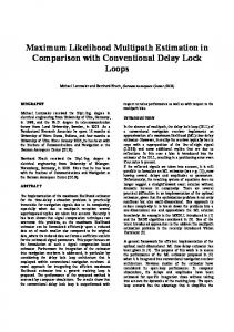
II. M ODEL AND F RAMEWORK Fig. 1 illustrates a general network topology, in which a node represents a computer or a subnet (a collection of computers). A connection between any two nodes in the network is called a path, which may consist of several links — direct connections between two nodes without intermediate nodes. A packet is a unit of data of bits. Information is exchanged by sending packets along a path from a source node to destination node(s).
t
bne
Su
Backbone
LAN
Fig. 1. An illustration of Internet topology
2
Let X = (X1 , ..., XJ )0 be a J dimensional random vector, which reflects the network dynamics of interest, e.g., link delay, traffic flow counts at a particular time interval. Let Y = (Y1 , ...,YI )0 be an I dimensional measurement vector. The goal of the network tomography is to estimate X from the observed Y. As in Coates et al. [7], such network tomography problems can be approximately (or exactly) represented by a linear equation: Y = AX, (1) where A is a known I × J routing matrix, determined by the network topology and the routing table at each router in the network. In this paper, we restrict ourselves to a fixed routing scheme and ignore the possibility of the dynamic routing; thus, A is a fixed 0-1 matrix. It is worth noting that we assume that there is no measurement or any other errors in (1) to further simplify the model. Equation (1) reveals the aggregative nature of network measurements, and so the estimation of the distribution of X is an inverse problem. In a general network tomography scenario, A is not a full rank square matrix, where typically I � J. Hence some constraints have to be introduced to ensure the identifiability of the model. A key assumption of the general network tomography model is that all components of X are independent of each other. Such an assumption does not hold strictly in a real network due to the temporal and spatial correlations between network traffic, but it is a good first-step approximation. Furthermore, we assume that X j ∼ f j (θ j ), j = 1, ..., J,
(2)
where f j is a density function with θ j being its parameter. Then the parameter of the whole model is θ = (θ1 , ..., θJ ). Throughout the paper, let Y1 , ..., YT be the observed data vectors at T consecutive time points or intervals, and X1 , ..., XT be the corresponding unobserved network performance quantities of interest and Yti , Xt j be the ith and jth element of Yt and Xt respectively. X1 , ..., XT (and hence Y1 , ..., YT ) are assumed to be identical independent distributed (i.i.d.). To deal with the nonstationary nature of the data, we use a local likelihood approach as employed in Cao et al. [5] by assuming that observations within a small moving time window are i.i.d. Now we are ready to construct the pseudo likelihood for the general network tomography model specified in (1). A. Subproblem Forming and Pseudo Likelihood Construction To obtain the pseudo likelihood for model (1), subproblems are formed by selecting some pairs of rows from the routing matrix A. In this paper, we select all possible pairs, but a subset can be judiciously chosen to reduce the computation. We first devise this approach for the multicast internal delay inference problem, which, after decomposition, is equivalent to the delay inference problem in the unicast framework [8]. We then generalize it to the general network tomography model (1), for which we will now present the construction of the pseudo likelihood. Let S denote the set of subproblems by selecting all possible pairs of rows from the routing matrix A: S = {s = (i1 , i2 ) : 1 ≤ i1 < i2 ≤ I}. Then for each subproblem s ∈ S, we have Ys = A s Xs ,
(3)
where Xs is the vector of network dynamic components involved in the given subproblem s, As is the corresponding subrouting matrix, and Ys = (Yi1 ,Yi2 )0 is the corresponding observed measurement of s. For later use, we introduce two notations here: given s, J s = { j : the jth element of X is involved in s }; given j, S j = {s : the jth element of X is involved in s }. Let θ s be the model parameter of the subproblem s, and p (Ys ; θ s ) be its marginal likelihood function. Then for the observed measurement vector Y, the pseudo log-likelihood function is defined as s
L p (Y; θ ) = ∑ logl s (Ys ; θ s ),
(4)
s∈S
where l s (Ys ; θ s ) = log ps (Ys ; θ s ) is the log-likelihood function of subproblem s. Given observed independent data vectors Y1 , ..., YT , let Xs1 , ..., XsT and Ys1 , ..., YsT , respectively, be the corresponding unobserved and observed data vectors for subproblem s. The overall pseudo log-likelihood function is then T
LTp (Y1 , ..., YT ; θ ) = ∑ L p (Yt ; θ ).
(5)
t=1
Maximizing the pseudo likelihood function gives the maximum pseudo likelihood estimate (MPLE) of parameter θ . Often one seeks to solve the following pseudo likelihood equation:
∂ p L (Y1 , ..., YT ; θ ) = 0. ∂θ T
(6)
To construct a pseudo likelihood function, selecting three or more rows each time may also be reasonable, but there is a trade-off between the computational complexity incurred and the estimation efficiency achieved by taking more dependence structures into account. Our experience with the two examples shown later suggests that selecting two rows each time gives satisfactory results while keeping the computational cost reasonable. B. Asymptotic Properties of MPLE Consistency and asymptotic normality are basic properties of MLE. Under some very general conditions, consistency and asymptotic normality of MPLE can also be obtained. In the rest of the paper, let θ0 be the true parameter in the model defined in (1) and (2), and θ0s be the true parameter of a subproblem s. Theorem 1: (Consistency) For the network tomography model defined in (1) and (2), assume the following conditions are satisfied: A1) L p (Y; θ ) is distinct, i.e., for any θ1 6= θ2 , there exists a set ∆ in the sample space RI , such that Pθ0 (∆) > 0 and for all Y ∈ ∆, L p (Y; θ1 ) 6= L p (Y; θ2 ); A2) The parameter space contains an open interval ω of which the true parameter θ0 is an interior point; A3) LTp (Y1 , ..., YT ; θ ) is differentiable with respect to θ . The pseudo likelihood equation (6) has a unique solution in ω almost surely when T → ∞.
3
Then the pseudo likelihood estimate θ˜Tp is consistent, i.e., θ˜Tp → θ0 in probability as T → ∞. For asymptotic normality, stronger conditions are needed to ensure the second order expansion in the neighborhood of the true parameter θ0 . Assume that the pseudo log-likelihood p function LT (Y; θ ) is twice continuously differentiable. Let H(θ ) = Eθ0 (∇2 L p (Y ; θ )) and B(θ ) = Varθ0 (∇L p (Y ; θ )). Theorem 2: (Asymptotic normality) In additional to the assumptions specified in Theorem 1, suppose the following conditions are also satisfied: B1) LTp (Y1 , ..., YT ; θ ) is twice continuously differentiable with respect to θ . In addition, expectation and differentiation operations of LTp (Y1 , ..., YT ; θ ) can be interexchanged; B2) With probability approaching 1, the Hessian matrix ∇2 LTp (Y1 , ..., YT ; θ ) is invertible in a small open interval ω around the true parameter θ0 as T → ∞; B3) For the same ω , ∇2 LTp (Y1 , ..., YT ; θ ) → H(θ ) in distribution uniformly for θ ∈ ω . Then the maximum pseudo likelihood estimate θ˜Tp is strongly consistent and as T → ∞, √ T (θ˜Tp − θ0 ) → N(0,C(θ0 )) in distribution, where C(θ ) = H(θ )−1 B(θ )H(θ )−1 . Since almost identical proofs can be found in [15] or [23], proofs of Theorems 1 and 2 are omitted. In the later sections, direct applications of Theorems 1 and 2 lead to Theorems 3 and 4. In their proofs, the following observations from [23] are used to check the conditions in Theorems 1 and 2: 1) The uniformly convergence of ∇2 LTp (Y1 , ..., YT ; θ ) to H(θ ) in the open neighborhood ω of θ0 can often be verified by checking ∂ 3L
p
that E ∂ θ j ∂ θ T∂ θ is bounded in ω , which holds for most analytic k
l
functions LTp ; 2) With necessary regularity conditions, the invertibility of the Hessian matrix ∇2 LTp (Y1 , ..., YT ; θ ) is ensured by the convexity of E∇2 LTp (Y; θ ) at θ0 for both multicast and OD inference problems. C. Pseudo EM Algorithm Maximizing the pseudo function leads to the MPLE, but often the pseudo likelihood equation (6) cannot be solved analytically; hence, a numerical optimization algorithm has to be adopted. The EM algorithm [11] is a well-known method for maximizing the likelihood function numerically. We use an pseudo-EM (an EM like algorithm) to maximize our pseudo likelihood functions. Let l s (Xs ; θ s ) be the log-likelihood function of a subproblem s given the unobserved complete data Xs . Let θ (k) be the estimate of θ obtained in the kth step; then the objective function Q(θ , θ (k) ) to be maximized over θ in the (k + 1)th step of the pseudo-EM algorithm is defined as T
Q(θ , θ (k) ) = ∑ ∑ Eθ s(k) (l s (Xts ; θ s )|Yts ) ,
(7)
s∈S t=1
which is obtained by assuming the independence of subproblems in the expectation step. As holds for the EM algorithm,
we have the following result for the pseudo-EM algorithm: during pseudo-EM iteration steps, the pseudo log-likelihood function LTp (Y1 , ..., YT ; θ ) is non-decreasing; moreover, if LTp is unimodal, then the pseudo-EM algorithm will converge to the unique maximum point. One needs to note that even though Theorem 1 and 2 guarantee the consistency and asymptotic normality of MPLE, the pseudo-EM algorithm may fall into a local maxima and hence not converge to the global maximum point. This problem occurs with any EM-like algorithms. On the other hand, for the two examples below, the proposed pseudo-EM algorithm is well-behaved, i.e., the algorithm actually finds the global maxima in most of the simulation and real data experiments.
III. A PPLICATIONS
OF
P SEUDO L IKELIHOOD E STIMATION
A. Example: Multicast Inference of Internal Delay Distribution Packet link delay is a major indicator of the network performance. Two different approaches have been used for link delay monitoring: internal and external. The internal approach directly measures the delays at link-level interfaces, while the external approach monitors delays through end-to-end measurements. The Multicast-based Inference of Network-internal Characteristics (MINC) Project [1] pioneered the use of multicast probing for network delay distribution estimation. The choice of end-to-end measurement through multicast probing is due to the limitations of the internal approach: (1) the collaboration between internal routers is not always available; (2) an extra heavy load burden might be caused by the probing process. A similar approach through unicast end-to-end measurements can be found in [8], but unicast methods suffer from scalability issues when large networks are of interest. Here we use the multicast-based external approach to estimate internal link delay distributions. Consider a general multicast tree depicted in Fig. 2. Each node is labeled with a number; we adopt the convention that link i connects node i to its parental node. Each probing packet with a time stamp sent from root node 0 will be received by all end receiver computers 4–7. For any pair of receivers, each packet experiences the same amount of delay over their common path. For instance, copies of the same packet received at receiver 4 and 5 experience the same amount of delay on their common links 1 and 2. Measurements are made at end receivers, so only the aggregated delays over the paths from root to end receivers are observed. Due to the aggregation of the measured delays, the network tomography model defined in (1) can be naturally applied to estimate the internal delay distribution. For each probing packet, X is the vector of unobserved delays over each link, and Y is the vector of observed path-level delays at each end receiver. A is an I × J routing matrix determined by the multicast spanning tree, where I is the number of end receivers and J the number of internal links. For the multicast tree depicted in Figure 2(a),
4
0
Root
Root
1 m
m
3
2
4
6
5
R1
7
R2
R3
R3
R1
(a)
(b)
Fig. 2. (a) An arbitrary virtual multicast tree with four receivers; (b) Psuedo Likelihood Decomposition: a virtual two-leaf multicast tree is formed by only considering a pair of end receivers (R1 ,R2 ).
the complete data Xs1 , ..., XsT is
(1) can be spelled out as: 1 Y1 Y2 1 Y3 = 1 Y4 1
1 1 0 0
0 0 1 1
1 0 0 0
0 1 0 0
0 0 1 0
X 1 0 X2 0 , 0 ... 1 X7
where Y1 , ...,Y4 are the measured delays at end receivers 4, ..., 7 and X1 , ..., X7 are the delays over internal links ending at nodes 1,..., 7. Each link has a certain amount of minimal delay (overhead), which is assumed to be known beforehand. After compensating the minimal delay of each link, a discretization scheme is imposed on link-level delay by Lo Presti et al. (1999) such that X j takes finite possible values {0, q, 2q, ..., mq, ∞}, where q is the bin width and m is a constant. Assume q is known, so without loss of generality, set q = 1. Therefore, each X j is a independent multinomial variable with with θ j = (θ j0 , θ j1 , ..., θ jm , θ j∞ ). When the delay is infinite, it implies the packet is lost during the transmission. The choice of m enables us to decide how fine we want to approximate the true delay distributions. In order to ensure identifiability, we only consider canonical multicast trees [17] defined as those satisfying
θ j0 = P(X j = 0) > 0, j = 1, ..., J, i.e., each individual packet has a positive probability to have zero delay over any internal link. For the problem of multicast delay inference through end-toend traffic, the maximum likelihood method is usually infeasible, because its likelihood function involves finding all possible internal delay vectors x given an observed delay vector y, and we can show that the computational complexity grows at a non-polynomial rate. Although Lo Presti et al.’s recursive algorithm [17] is a computational efficient method in estimating internal delay distributions, it suffers from some performance drawbacks. But we can apply the pseudo likelihood approach to this problem. In this case, each row of the routing matrix A corresponds to an end receiver in the multicast tree, and subproblems are formed by choosing two end receivers each time as illustrated in Fig. 2(b). 1) Parameter Estimation through Pseudo-EM: For a given subproblem s, each component of Xs is an independent multinomial random variable, so that the log-likelihood function given
l s (Xs1 , ..., XsT ; θ s ) =
∑ ∑ nsjl log(θ jl ),
j∈J s l
where θ jl = P(X j = l), nsjl = ∑t 1{Xts j =l} .
Let θ (k) be the parameter estimate obtained in the kth step of Pseudo EM, then according to (7), the target function to be maximized in the (k + 1)th step is ! T (k) Q(θ , θ ) = ∑ ∑ ∑ log(θ jl )Eθ s(k) ∑ 1{Xts j =l} Yts . s s∈S j∈J
t=1
l
E-step: compute
nˆ jl = ∑ Eθ s(k) s∈S
M-step: update θ (k) by (k+1)
θ jl
=
! ∑ 1(Xts j = l) Yts ; T
t=1
nˆ jl , where R = {0, 1, ..., m, ∞}. ∑r∈R nˆ jr
The initial value of the pseudo-EM algorithm can be chosen arbitrarily. We find that small starting values may have difficulties to increase even when the true parameter θ0 is not small. (0) A uniform distribution, i.e., θ jl = 1/(m + 2) for all possible j and l, is used as the starting point for our simulations below. Such a uniform starting point gives satisfactory results. Let P be the average number of links per path, then the overall computational complexity of each step of the pseudo-EM algorithm is O(m3 I 2 P2 ). Meanwhile, specializing Theorem 1 and 2 to this example gives the consistency and asymptotic normality of the MPLE. Theorem 3: Assume that θ0 is in the interior of the parameter space (note that it implies that the multicast tree is a canonical tree.) Let θ˜Tp be the internal delay distribution estimate through maxiizing likelihood, then θ˜Tp is a consistent estima√ the pseudo p tor, and T (θ˜T − θ0 ) converges in distribution to a multivariate normal random variable as T → ∞. 2) Experimental results: In order to assess the performance of the pseudo likelihood methodology, model simulations are carried out on a 4-leave multicast tree depicted in Fig. 2(b). Due to its small size, the MLE method is implemented for this multicast tree, so we can compare the performance of MPLE
5
0.0
L−1 Error Norm 0.5 1.0
1.5
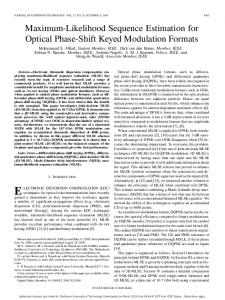
with that of MLE and recursive algorithm for this simulation. The initial value of the EM algorithm in implementing MLE is also set to be the uniform distribution. For each link, the bin size parameter m is set to be 14. During each simulation, 2000 i.i.d. multicast delay measurements are generated with each internal link having an independent discrete delay distribution. Fig. 3 shows the delay distribution estimates of three arbitrarily selected links along with their true delay distributions in one such experiment. The plot shows both MPLE and MLE capture most of the link delay distributions and their performace is comparable, while the recursive algorithm sometimes gives estimate far from the truth. Still we can see sometimes both MPLE and MLE have estimates quite different from the true probability. Mainly, this is due to that the number of parameters needs to be estimated, 7 × 16 = 112, is large, and moreover by its nature such an inverse problem is ill-posed. Fig. 4 shows the L1 error norm of MLE, MPLE and recursive estimate for each link, as averaged over 30 independent simulations. For each link, the L1 error norm is simply the sum of the absolute differences between probability estimates and the true probabilities. As a common measure of the performance of density estimates, the L1 error norm enjoys several theoretical advantages as discussed in [18]. The plot shows that MLE and MPLE have a comparable estimation performance for tracking link delay distributions, while the recursive algorithm has much larger L1 errors on all links. Moreover, we can see that MPLE has smaller standard deviations (SD) in terms of L1 error than MLE on all links, implying that MPLE is more robust than MLE. This is probably because the pseudo likelihood function, which is a product of less complex likelihood functions on subproblems, has a nicer surface than the full likelihood function [4].
1
2
3
4 Links
5
6
7
Fig. 4. Link L1 error norm averaged over 30 simulations: solid line is MPLE, dashed line is MLE, and dotted line is recursive algorithm. For each link, the vertical bar shows the SD of L1 error norm for the given link.
B. Example II: Origin-Destination Matrix Inference The origin-destination (OD) matrix, whose elements are the byte counts of traffic between all origin-destination pairs in a network, is a key input to any routing algorithm, since the link weights of the Open Shortest Path First (OSPF) routing protocol are related to the traffic on the path. Two approaches exist to carry out the OD matrix estimation: direct and indirect. The
direct approach via router softwares, such as Netflow supported by Cisco routers, is described in [12]. Indirect approaches use link traffic counts at router interfaces, which are much easier to obtain. Hence, indirect methods based on the observed link counts at router interfaces have been more intensively studied ([22], [21], [19]). Vardi [22] was the first to investigate this problem. Assuming i.i.d. Poisson distributions for the OD traffic byte counts on a general network topology, he specifies the identifiability of the Poisson model and develops an EM algorithm to estimate Poisson parameters in both deterministic and Markov routing schemes. In order to ease the difficulty in implementing the EM algorithm, he proposes a moment estimation method and briefly discusses the normal model as an approximation to the Poisson model. Two related works treat the special case involving a single set of link counts: Vanderbei and Iannone (1994) apply the EM algorithm; Tebaldi and West (1998) is a followup on Vardi (1996) with a Bayesian perspective and a Markov Chain Monte Carlo implementation. With real network data, Cao et al. [5] revise the Poisson assumption and propose a normal model. They also address the non-stationarity of the network OD traffic. Their methodology is validated through comparisons with directly collected (but expensive) OD traffic in a simple network at Lucent Technologies depicted in Fig. 5. Our pseudo likelihood method is based on their normal model. Next we briefly review the normal model and their methodologies in OD matrix inference. The network tomography model specified by (1) is applicable to the OD matrix inference through link traffic counts. Recall that Y = (Y1 ,Y2 , ...,YI )0 is the vector of observed traffic byte counts measured on each link interface during a given time interval and X = (X1 , X2 , ..., XJ )0 is the corresponding vector of unobserved true OD traffic byte counts at the same time period. X is called OD traffic matrix, even though it is arranged as a column vector for notational convenience. Under a fixed routing scheme, Y is determined uniquely by X through the I × J routing matrix A, in which I is the number of measured incoming/outgoing unidirectional links and J is the number of possible OD pairs. Each column of A is associated with an OD pair and indicates which links are used to carry traffic for that pair of nodes, while each row corresponds to an observed link traffic. For instance, the routing matrix A (0 for entries not shown) of the single-router network depicted in Fig. 5(b) is orig-1 1 1 1 1 orig-2 1 1 1 1 1 1 1 1 orig-3 1 1 1 1 orig-4 A = dest-1 1 , 1 1 1 1 1 1 dest-2 1 1 1 1 1 dest-3 1 1 1 1 dest-4
where the first column of A indicates that two links (rows of A) orig1 and dest1 contain the OD traffic from fddi to itself. The first row of A means that the traffic originated from node fddi consists of 4 pairs of unobserved OD pair traffic originated from fddi and destined to all other 4 nodes (including itself). In the normal model [5], each component of X is assumed to be independent normally distributed, satisfying the following mean-variance relationship: X j ∼ N(λ j , φ λ jc ) independently,
6
pseduo
true
0 Link 1
0.2
mle
5
10
recursive
15
Link 2
Link 4
Probability
0.15
0.1
0.05
0
0
5
10
15
0
5
10
15
Fig. 3. Delay distribution estimates of 3 arbitrarily selected internal links: Link 1, Link 2 and Link 4. Solid step function is the true distribution, dash line with circle is MPLE, dotted line with triangle is MLE, and dash line only is recursive estimate.
2
Firewall
Router1 Router2
switch
Gateway
Router3 Router4
internet
Switch
Firewall
r4-local 1 fddi
Router1
gw1
switch
local 3
Router4
gw3
Gateway
fddi local corp
r4-others gw-others Router5
corp
router5
4
(a)
(b)
gw2
(c)
Fig. 5. (a) A Simple Router Network at Lucent Technologies, (b) Network Topology around Router 1, (c) A two-router Network around Router 4 and Gateway.
where φ is a positive scalar applicable to all OD pairs and c is a power constant. It implies that Y = AX ∼ N(Aλ , AΣA0 ), where λ = (λ1 , · · · , λJ ) and Σ = φ diag(λ1c , · · · , λJc ). So the parameter of the full model is θ = (φ , λ ). The mean-variance relationship is a crucial assumption to ensure the identifiability of the normal model. It implies that an OD pair with large traffic byte counts tends to have large variance with the same scale factor φ . For the power constant c, both c = 1 and 2 work well with the Lucent network data as shown in [5], [6]. Because c = 1 or c = 2 give similar results, in this paper, we use c = 1 as done in [6]. But note that the pseudo likelihood method we will propose later can deal with c = 2 without any additional technical difficulties. Cao et al. [5] also address the non-stationarity of network traffic by a local likelihood model, i.e., for any given time interval t, analysis is based on observations within a symmetric window of size w around t. Within each window, observations are assumed to be independent. Maximum likelihood estimate is carried for each window via a combination of EM algorithm and a second-order optimization routine. In order to estimate the underlying true OD traffic x, the conditional expectation Eθˆ(Xt |Yt , Xt > 0) is computed as an initial estimate of x. Then an iterative proportional fitting (IPF) algorithm [10], widely used in contingency table analysis to adjust table to match the observed margins, is employed to enforce the linear constraint y = Ax to obtain the final estimate of OD traffic x. In [5], to smooth the parameter estimate, a random walk model is applied
to the parameter λ ’s and φ over the sliding time windows. For the normal model, the computational complexity is high. Let n be the number of edge nodes in a network, as discussed in [6], the computational complexity of the full MLE is O(n5 ) after exploiting sparse matrix calculation. Hence, the pseudo likelihood approach is applied to the above normal model. Comparisons will be made between full and pseudo likelihood with respect to the computational complexity and estimation efficiency in later sections. 1) Parameter Estimation through Pseudo-EM: For each subproblem s, Ys is the vector of observed traffic byte counts and As is the sub-routing matrix. Xs is the vector of OD pair traffic counts involved in s. Let λ s , Σs be the mean vector and covariance matrix of Xs respectively. The parameter of the subproblem s is then θ s = (φ , λ s ). The log-likelihood function for subproblem s given complete data Xs1 , ..., XsT is l s (Xs1 , ..., XsT ; θ s ) = −
T 1 T s s log |Σs |− ∑ (Xts − λ s )0 Σ−1 s (Xt − λ ). 2 2 t=1
Let θ (k) be the parameter estimate in the kth step. According to (7), the objective function to be maximized in the (k + 1)th step is � � � s(k) Q(θ , θ (k) ) ∝ − ∑ T log |Σs | + tr(Σ−1 ) s R s∈S T
+ ∑ (mt t=1
s(k)
s(k)
− λ s )0 Σ−1 s (mt
− λ s)
�
(8)
7
s(k)
where mt have s(k)
mt
Rs(k) s(k)
and r j
= Eθ s(k) (Xts |Yts ) and Rs(k) = Varθ s(k) (Xts |Yts ). We (k)
(k)
= λ s(k) + Σs As0 (As Σs As0 )−1 (Yts − As λ s(k) ), (k)
(k)
(k)
(k)
= Σs − Σs As0 (As Σs As0 )−1 As Σs , s(k)
and mt j
are, respectively, the elements in Rs(k) and
s(k)
mt
corresponding to OD pair j. Let d j be the number of elements in S j , and (k) aj (k)
bj
= =
1 dj
∑
s(k) rj +
s∈S j
! 1 T s(k) 2 ∑ (mt j ) , T t=1
T 1 s(k) m , ∑ ∑ T d j s∈S j t=1 t j
then it can be shown that the ∂ Q/∂ θ (θ , θ (k) ) = 0 is equivalent to (k)
system
equation
λ j2 + φ λ j − a j = 0, j = 1, ..., J
(9a)
∑ (λ j − b j
(9b)
J
(k)
) = 0.
j=1
(k)
(k)
E-step: Compute coefficients a j and b j . Compared with the full likelihood method, the computation is much faster because As Σs As0 is simply a 2 × 2 matrix. So there is no need to invert a very high dimensional matrix as the full likelihood method does. M-step: Solve (8). Equation (8a) shows quadratic constraint between λ j and φ . In conjunction with these solutions, (8b) boils down to a monotonic functional constraint on φ , therefore fast searching algorithms are available to solve these equations. Because the cost of the E-step is relatively high, a Multiple-Step Gradient EM algorithm (a natural extension to Lange’s Gradient EM algorithm [14]) is employed to solve these equations only roughly. The starting point θ (0) = (λ (0) , φ (0) ) can be quite arbitrary for the pseudo-EM algorithm. For the OD matrix inference experiments below, we adopt the same initial value used in [5], such that λ (0) is a constant vector with each component to be T 10 Yt /(T 10 A1) and φ (0) = Var(Yti )/E(Yti ), where the sam∑t=1 ple variance and expectation is computed by pooling all Yti together. Such starting point gives very stable performance for the Lucent and simulated data set. For a network with n nodes, the number of observed unidirectional links I is O(n), and the number of OD pairs J is n2 . Assuming√that the average number of links between an OD pair is O( n), it can be shown that on average each subproblem involves O(n1.5 ) OD traffic pairs, thus for the n2 subproblems, the overall computational complexity of each step of the pseudo-EM algorithm is O(n3.5 ). Compared with the complexity of the full likelihood O(n5 ), the pseudo likelihood approach reduces the computational complexity considerably. Moreover, the pseudo likelihood approach fits in the framework of distributed computing, which can be advantageous for practical applications. Therefore, the pseudo likelihood approach is
more scalable to larger networks. As future research, we plan to use only a subset of subproblems in parameter estimation to further reduce the computational complexity. Theorem 4: Let B be an [I(I + 1)/2] × J matrix whose rows are the rows of A and the component-wise products of each different pair of rows from A. If B is of full column rank, then the model is identifiable. Let θ˜Tp be the parameter estimate through pseudo likelihood, then θ˜Tp is a consistent estimator and when √ p T → ∞, T (θ˜T − θ ) converges in distribution to a multivariate normal random variable. 2) Experimental results: Two types of experiments are conducted to assess the performance of the pseudo likelihood method. First, we consider a small real network at Lucent Technologies depicted in Fig. 5(b). For this 4-node network, there are 4 incoming and 4 outgoing links and the total number of OD pairs J is 16. For this network, the true OD traffic counts are collected through Netflow in every 5 minutes, so we can compare the estimated traffic counts (derived from the parameter estimates) with the true traffic counts. In order to have good comparison, we use the the data collected on Feb 22, 1999, the same day used in [5], which consists of 288 data points. We adopt the same window size 11 from Cao et al. for the local moving i.i.d. model to capture the time varying nature of the network traffic. Fig. 6 shows the MPLE of λ , the mean OD traffic, along with its MLE estimate. For comparison, the 11-points moving average of true OD traffic counts are also plotted. We can see that both pseudo and full likelihood methods capture the dynamics of the OD traffic counts quite well. For estimating the actual time-varying OD traffic counts Xt , estimates of OD network traffic counts near high peaks usually have a relatively smaller error rate. In order to exhibit smallscale features, a zoomed-in version of the OD traffic counts estimate with its vertical axis magnified by a factor of 20 is shown in Fig. 7. The plot demonstrates that both pseudo and full likelihood methods have quite comparable performance even in error-prone small scales. The above computations are completed using R 1.5.0 [13] on a 1G Hz laptop. In producing Fig. 6, it takes about 12 seconds for computing the MPLE, and about 49 seconds for the MLE. In the pseudo likelihood approach, the computation of coeffi(k) (k) cients ai and bi is done by C codes because the performance of R will be severely affected by multiple loops introduced by dealing with numerous subproblems. Similarly, EM algorithm is used to compute MLE, and the only difference between EM and pseudo-EM in this problem is how they compute coeffi(k) (k) cients ai and bi . In the E-step of EM for the full likelihood method, one matrix inversion and a few matrix multiplications are needed. All operations can be done in R very efficiently, hence the introduction of C codes in the E-step of the full likelihood method will barely speed up its execution. Second, in order to assess the performance of MPLE more thoroughly, simulations are carried out on some larger networks through network simulator (NS) [16]. OD traffic is simulated on a two-router network depicted in Fig. 5(c). Every link is configured to have a capacity of 1.5Mbps and a propagation delay of 10ms with default drop tail queueing management. Each OD pair is assigned a bit rate; during the simulation, the node generates exponential on-off UDP packets to the destination node
8
1M
observed 50 100 150 200 250
pseudo
0
mle 50 100 150 200 250
dst fddi
dst switch
dst local
dst corp
total
corp>fddi
corp>switch
corp>local
corp>corp
src corp
800K 600K 400K 200K 0 1M 800K 600K 400K
Traffic counts (Byte/Sec)
Fig. 6. Mean OD traffic estimates λˆt obtained from pseudo and full likelihood methods for 4 nodes network around Router1 against the moving average of the true OD traffic. Marginal traffic is shown in side panels.
0
200K 1M
local>fddi
local>switch
local>local
local>corp
src local
switch>fddi
switch>switch
switch>local
switch>corp
src switch
0
800K 600K 400K 200K 0
1M 800K 600K 400K 200K
fddi>fddi
1M
fddi>switch
fddi>local
fddi>corp
src fddi
800K 600K 400K 200K 0 0
50 100 150 200 250
0
50 100 150 200 250 Hours of day
0
50 100 150 200 250
0
observed 50 100 150 200 250
pseudo
0
mle 50 100 150 200 250
dst fddi
dst switch
dst local
dst corp
total
corp>fddi
corp>switch
corp>local
corp>corp
src corp
Traffic counts (Byte/Sec)
50K 40K 30K 20K 10K 0
50K 40K 30K 20K 10K 0 local>fddi
local>switch
local>local
local>corp
src local
switch>fddi
switch>switch
switch>local
switch>corp
src switch
50K 40K 30K 20K 10K 0 50K 40K 30K 20K 10K 0 fddi>fddi
fddi>switch
fddi>local
fddi>corp
src fddi
50K 40K 30K 20K 10K 0 0
50 100 150 200 250
0
50 100 150 200 250 Hours of day
0
50 100 150 200 250
9
Fig. 7. OD traffic counts estimates ˆ txobtained from pseudo and full likelihood methods against the true OD traffic counts for 4 nodes network around Router1. The plot has been zoomed in by a factor of 20 to show small-scale features.
0
10
with the given rate. The burst time of the generating process is set to be 20ms and idle time 120ms. Background traffic consists of a mixture of exponential or pareto on-off sources using TCP or UDP. Each background connection is randomly attached to an OD pair and has random bit rate and start stop times. Flow monitor is utilized to collect flow, i.e., OD traffic statistics. The simulation lasts 288 seconds: every second represents a 5-minute interval in a 24 hours long data collection. In Fig. 8, we show the results of byte count estimates on 9 selected OD pairs (from 3 nodes to another 3 nodes). Those pairs are chosen because they have larger estimation errors compared with other pairs. From the plot, we see that both pseudo and full likelihood methods capture the dynamics of the simulated OD traffic under the zoomed-in scale. It takes about 18 seconds to compute the MPLE, while it takes around 88 seconds to compute the MLE. An even larger simulation is carried out on the Lucent network illustrated in Fig. 5(a), which comprises 21 end nodes and 27 links. The OD traffic estimate plots (not shown) once again show that both MPLE and MLE capture the dynamic of the simulated OD traffic and yield similar results. The execution times of pseudo and full likelihood methods are 2.5 minutes and 39.9 minutes respectively. The comparison of execution times between MLE and MPLE exhibits that the pseudo likelihood approach speeds up the computation without losing much estimation performance, so it is more scalable to larger networks. 0 gw3>r4local
observed 50 100
150
pseudo 200
250
mle
gw3>switch
gw3>gw2
40K
for large network problems. We believe more decomposition schemes may emerge to solve other network tomography problems beyond the two special cases demonstrated here. ACKNOWLEDGMENTS We would like to thank two anonymous referees for their constructive comments on the previous versions of this paper. We also would like to thank Jonathan Grib, Mike Last, and Dave Graham-Squire for very helpful comments on the presentation of the paper. Last, but not least, we thank Jin Cao and Scott Vander Wiel for sharing the collected traffic data on the Lucent network and their Splus codes. A PPENDIX For notational convenience, given observed Y1 , ..., YT , let LTp (θ ) be a shorthand for the pseudo log-likelihood function LTp (Y1 , ..., YT ; θ ), and l s (θ s ) for l s (Ys1 , ..., YsT ; θ s ). Proof of Theorem 3: We proceed by verifying the conditions in Theorems 1 and 2. The true parameter θ0 is assumed in an open interval ω of the parameter space (condition A2). It is easy to show that the pseudo likelihood function L p (Y, θ ) is infinitely differentiable, and its expectation and derivative operations can be inter-exchanged (condition B1). If we can show the distinctiveness of L p (Y, θ ) (condition A1) and the pseudo log-likelihood function LTp is strictly convex in a neighborhood of the true parameter θ0 as T → ∞ (condition B2), then we can conclude that the pseudo likelihood equation (6) has a unique solution in a neighborhood of θ0 almost surely (condition A3). Therefore, the MPLE is consistent by Theorem 1. Also because ∂ 3Lp
20K
0 r4others>switch
r4others>gw2
Traffic counts (Byte/Sec)
r4others>r4local
40K
20K
0 router5>r4local
router5>switch
router5>gw2
40K
20K
0 0
50
100
150
200
250
0
50
100
150
200
250
Hours of day
Fig. 8. OD traffic count estimates ˆ tx on selected OD pairs for NS simulated data on a two-router network depicted in Fig. 5(c). Each panel shows the pseudo and full likelihood methods against the observed simulated OD traffic.
IV. C ONCLUSIONS In this paper, we proposed a pseudo likelihood approach to the network tomography problem and included two special cases (multicast link delay estimation and OD traffic estimation) to demonstrate the potential of the proposed approach. In the two special cases, the MPLE shows strengths through its estimation efficiency and manageable computational complexity. Even though the basic idea of divide-and-conquer is not new, it is very powerful when combined with pseudo likelihood
θ0 is in the interior of the parameter space, ∂ θ j ∂ θ T∂ θ is continuk l ous hence bounded in a neighborhood of true parameter θ 0 and so is its expectation (condition B3). It follows the normality of the MPLE by Theorem 2. First, in order to proof the distinctiveness of L p (Y, θ ), we need to show that if L p (Y, θ1 ) = L p (Y, θ2 )
(10)
holds for all possible values of Y, then θ1 = θ2 . Taking expectation with respect to Pθ1 , Equation (9) becomes the sum of Kullback-Leibler (KL) divergences over subproblems being zero. So each term is zero and hence the log-likelihood is equal for each subproblem: l s (Ys , θ1s ) = l s (Ys , θ2s ). For each subproblem, it is easy to show that its three virtual sub-paths, e.g., Root → m, m → R1 and m → R3 in Fig. 2(b), have the same delay distribution when the true parameter is θ1 or θ2 . Now we visit all sub-paths from top to down to show that each internal link has the same distribution under θ1 and θ2 . For instance, consider the multicast tree depicted in Fig. 2(a). Link 1 has the same distribution under θ1 and θ2 because it is a sub-path of s = (1, 4) (subproblem formed by end nodes 4 and 7). Also we know that sub-path 0 → 2 has the same distribution under θ 1 and θ2 by considering subproblem s = (1, 2). Using the fact that the delay distribution for each sub-path is the convolution of its sub-link distributions, we know Link 2 has the same distribution by deconvolution. Repeating this process, we see that all
11
internal links have the same distribution under θ1 or θ2 . Hence we prove the distinctiveness of LTp (θ ). Second, we want to show LTp (θ ) is strictly convex in a neighborhood of the true parameter θ0 with probability approaching 1 when T goes to infinity. Because Y1 , ..., YT are i.i.d. copies of Y, we only need to prove that EL p (Y; θ ) is strictly convex at θ0 , i.e., the Hessian matrix −E∇2 L p (Y; θ0 ) = −E∇2 L p (Y; θ )|θ =θ0 is positive definite. Note that l s (Ys ; θ s ) is the true log-likelihood function of subproblem s with θ0s being its true parameter, we have E∇l s (Ys ; θ0s ) = 0, and that −E∇2 l s (Ys ; θ0s ) = Var∇l s (Ys , θ0s ) is a non-negative definite matrix. By observing that L p (Y; θ ) is a sum of log-likelihood functions of subproblems, we have E∇L p (Y; θ0 ) = 0 and the Hessian matrix −E∇2 L p (Y; θ0 ) is non-negative definite. What remains to be shown is that it is actually positive definite. Suppose there is a vector α , such that 0 = −α 0 E∇2 L p (Y; θ0 )α = ∑ Var(α 0 ∇l s (Ys , θ0s )) s∈S
then α 0 ∇l s (Ys , θ0s ) = 0 for any possible values of Y and s. Similarly we enumerate through all subproblems from top to down to show α = 0. For instance, consider the multicast tree depicted in Fig. 2(a) again. For subproblem s = (1, 4), α 0 ∇l s (Ys , θ0s ) = 0 implies that the components of α corresponding to Link 1 are all 0. Based on this information, that α 0 ∇l s (Ys , θ0s ) = 0 for subproblem s = (1, 2) implies the components of α corresponding to Link 2 are all 0. We repeat this process to show that all components of α are zero, i.e., the Hessian matrix is positive definite.
Proof of Theorem 4: For the OD traffic matrix inference problem, θ = (φ , λ ). Similar to Theorem 3, we only need to show the distinctiveness of LTp (θ ) and its convexity in a neighborhood of θ0 . The same KL-divergence argument in the proof of Theorem 3 shows LTp (θ1 ) = LTp (θ2 ) if and only if l p (θ1s ) = l p (θ2s ) for all s, so for distinctiveness, it is enough to show that l s (θ1s ) = l s (θ2s ) for all sub-problem s implies θ1 = θ2 . For a sub-problem s = (i1 , i2 ), let Bs be a 3 × J matrix, with the i1 th, i2 th rows of A being the first two rows and their component-wise product being the third row. Then l s (θ1s ) = l s (θ2s ) implies
φ 1 = φ 2 , B s λ1 = B s λ2 . Thus, we have Bλ1 = Bλ2 and φ1 = φ2 . Because B is of full column rank, Bλ1 = Bλ2 implies λ1 = λ2 . This establishes the distinctiveness of LTp (θ ). p Second, we want to show that LT (θ ) is strictly convex in a neighborhood of true parameter θ0 , i.e., the Hessian matrix −E∇2 L p (Y; θ0 ) is positive definite. Let α = (a, b), where a is a scalar and b is a J-dimensional vector. We can show that α E∇2 L p (Y; θ0 )α 0 = 0 is equivalent to α ∇l p (Ys ; θ0s ) = 0 for all possible values of Y and subproblem s. For each subproblem s,
and α ∇l p (Ys ; θ0s ) = 0 can be simplified as a = 0 and Bs b = 0. Thus, we have a = 0 and Bb = 0. Once again, that B is of full column rank implies b = 0, i.e., α = 0. It follows that the pseudo log-likelihood function LTp (θ ) converges to a convex function in a neighborhood of θ0 as T → ∞. R EFERENCES [1] Multicast-based Inference of Network-internal Characteristics (MINC), http://www.research.att.com/projects/minc/. [2] J. Besag. Spatial interaction and the statistical analysis of lattice systems. Journal of the Royal Statistical Society, Series B, 36(2):192–236, 1974. [3] J. Besag. Statistical analysis of non-lattice data. Statistican, 24(3):179– 195, 1975. [4] David Blackwell. Approximate normality of large products. Technical report, University of California at Berkeley, 1973. [5] J. Cao, D. Davis, S. Vander Wiel, and B. Yu. Time-varying network tomography: router link data. Journal of American Statistics Association, 95(452):1063–1075, 2000. [6] J. Cao, S. Vander Wiel, B. Yu, and Z. Zhu. A scalable method for estimating network traffic matrices. Technical report, Bell Labs, 2000. [7] M. Coates, A. Hero, R. Nowak, and B. Yu. Internet tomography. Signal Processing Magazine, 19(3):47–65, 2002. [8] M. Coates and R. Nowak. Network tomography for internal delay estimation, 2001. [9] D. R. Cox. Partial likelihood. Biometrika, 62:269–276, 1975. [10] I. Csisz´ar. I -divergence geometry of probability distributions and minimization problems. The Annals of Probability, 3(1):146–158, 1975. [11] A. Dempster, N. Laird, and D. Rubin. Maximum likelihood from incomplete data via the em algorithm. Journal of Royal Statististical Society B, 39:1–38, 1977. [12] A. Feldmann, A. Greenberg, C. Lund, N. Reingold, J. Rexford, and F. True. Deriving traffic demands for operational ip networks: Methodology and experience. IEEE/ACM Transactions on Networking, pages 265–279, June 2001. [13] Ross Ihaka and Robert Gentleman. R: A language for data analysis and graphics. Journal of Computational and Graphical Statistics, 5(3):299– 314, 1996. [14] K. Lange. A gradient algorithm locally equivalent to the em algorithm. Journal of the Royal Statistical Society, Series B, 57:425–437, 1995. [15] E. L. Lehmann and G. Casella. Theory of Point Estimation. SpringerVerlag, NY, 2nd edition, 1998. [16] ns (Network Simulator). http://www.isi.edu/nsnam/ns. [17] F. Lo Presti, N.G. Duffield, J. Horowitz, and D. Towsley. Multicast-based inference of network-internal delay distributions. Technical report, AT&T Laboratories and University of Massachustts, 1999. [18] D.W. Scott. Multivariate Density Estimation: Theory, Practice and Visulization. Wiley, Ney York, 1992. [19] C. Tebaldi and M. West. Bayesian inference on network traffic using link count data (with discussion). Journal of American Statistics Association, pages 557–576, June 1998. [20] Yolanda Tsang, Mark Coates, and Robert Nowak. Nonparametric internet tomography. In IEEE International Conference on Acoustics, Speech, and Signal Processing, Orlando, Florida, May 2002. [21] R. J. Vanderbei and J. Iannone. An EM approach to OD matrix estimation. Technical report, Princeton University, 1994. SOR 94-04. [22] Y. Vardi. Network tomography: Estimating source-destination traffic intensities from link data. Journal of the American Statistical Association, 91:365–377, 1996. [23] H. White. Estimation, Inference and Specification Analysis. New York: Cambridge University Press, 1994.
1 1 l s (Ys , θ s ) = − log|As ΣAs0 |− (Ys −As λ )(As ΣAs0 )−1 (Ys −As λ )0 , 2 2