MC-ANT: a Multi-colony Ant Algorithm Leonor Melo, Francisco Pereira, and Ernesto Costa Instituto Superior de Engenharia de Coimbra, 3030-199 Coimbra, Portugal Centro de Inform´ atica e Sistemas da Universidade de Coimbra, 3030-790 Coimbra, Portugal
[email protected] {xico,ernesto}@dei.uc.pt
Abstract. In this paper we propose an ant colony optimization variant where several independent colonies try to simultaneously solve the same problem. The approach includes a migration mechanism that ensures the exchange of information between colonies and a mutation operator that aims to adjust the parameter settings during the optimization. The proposed method was applied to several benchmark instances of the node placement problem. The results obtained shown that the multicolony approach is more effective than the single-colony. A detailed analysis of the algorithm behavior also reveals that it is able to delay the premature convergence. Key words: Ant Colony Optimization, Multiple colony, Node Placement Problem, Bidirectional Manhattan Street Network
1
Introduction
Ant Colony Optimization (ACO) is one of the most successful branches of swarm intelligence [4]. ACO takes inspiration from social insects such as ants. While foraging real ants deposit pheromone on the ground to guide the other members of the colony. ACO mimics this indirect way of communication. The first ant algorithms were proposed by [6], [7] as a multi-agent approach to solve difficult combinatorial optimization problems like the traveling salesman problem. Since then a wide range of variants were proposed and applied to different classes of problems (see [8] for an overview). In this paper we propose MC-ANT, a multi-colony ACO. The idea behind this approach is to allow for the simultaneous exploration of several search locations and to dynamically intensify the search on the most promising ones. Each colony maintains its own trail and set of parameters, but the most successful colonies transfer information to the worst ones. Specifically the trails of the worst colonies are periodically updated, which hopefully will help them to escape from local optima and move towards more promising locations. We illustrate our approach by addressing the problem of finding the optimal node assignment in a multi-hop Wavelength Division Multiplexing (WDM) lightwave network with a virtual Bidirectional Manhattan Street Network topology
2
Leonor Melo, Francisco Pereira, and Ernesto Costa
[16]. One advantage of this type of network is the ability to create a virtual topology different from the underlying physical topology. The assignment of the physical nodes to the virtual topology is a strong factor in the efficiency of the network. The results obtained are encouraging as they show the advantage provided by the existence of several colonies. Migration is able to enhance the algorithm performance without causing the convergence of the colonies to the same trail. The structure of the paper is the following: in sec. 2 we briefly describe Ant Colony Optimization algorithms and in sec. 3 we present the Node Placement Problem. Section 4 comprises the presentation of our multi-colony approach. Results from experiments are presented in sec. 5 and, finally, in sec. 6 we provide the main conclusions.
2
Ant Colony Optimization
In many species, an ant walking to or from a food source leaves a substance in the ground called pheromone. The other ants tend to follow the path where the pheromone concentration is higher [3]. [11] proved that this pheromone laying mechanism is used to guide the other members of the colony to the most promising trails. In an ACO algorithm, artificial ants use an artificial trail (together with some heuristic information) to guide them in the process of building a solution to a given problem. While the heuristic information is static the pheromone trail is updated according to the solutions found in previous iterations. Starting from an empty solution, components are probabilistically added one by one until a complete solution is obtained. Some heuristic knowledge can also be used to bias the choice. The specific formula used to select the next solution component depends on the ACO variant. The general ACO algorithm consists of three phases (see fig. 1). After the initialization and until some termination condition is met the following steps are repeated: each ant builds a solutions, the best(s) solution(s) are improved by a local search (this step is optional) and at last the pheromone trail is updated. set the parameters initialize the pheromone trail while termination condition not met do construct ant solutions apply local search (optional) update pheromone trail end_while
Fig. 1. The ACO metaheuristic
MC-ANT
2.1
3
ACO Algorithms
ACO algorithms have been applied to many problems. Examples are the applications to assignment problems, scheduling problems and vehicle routing problems [8]. Among other applications, ACO algorithms are currently state-of-the-art for solving the sequential ordering problem (SOP), the resource constraint project scheduling (RCPS) problem, and the open shop scheduling (OSS) problem [8]. Ant System (AS) [6], [7] was the first ACO algorithm. Since then some some variants have been derived, being the MAX-MIN Ant System (MMAS) [19] and Ant Colony System (ACS) [5] some of the most successful and most studied of them [8]. A common characteristic of ACS and MMAS is that they focus their search in a specific region of the search space [8]. We thus hope that by using an island model approach a bigger portion of the landscape can be covered. Our method is inspired in the ACS, partly because is considered the most aggressive of the two [8] and is able to find better solutions in short computation times, although it converges sooner to a suboptimal solution. We hope the multi-colony method helps avoiding the premature convergence while retaining the ability to reach good solutions fast. 2.2
Ant Colony System (ACS)
ACS tries to diversify the solutions landscape covered by the ants in an iteration by introducing a pheromone update during the construction step. At each decision point, each of the ants updates the trail by slightly decreasing the pheromone level of the component it just choose. The regular pheromone update at the end of each iteration considers only one ant, either the iteration best, the best-so-far or a combination of both. The formula used is (1) where Lbest is the quality of the solution found by the selected ant. { ρ (1 − ρ) · τij + Lbest if cij is in the solution τij = (1) τij otherwise The mechanism used to select the next component uses a pseudo-random proportional rule. Depending on the value of a parameter q0 the rule may favor either exploration or exploitation. 2.3
Multi-colony ACO
In multi-colony ant algorithms several colonies of ants cooperate in order to find good solutions for the problem being solved [18]. The cooperation takes place by exchanging information about good solutions. There are a few proposed multi-colony variants of the ACO. Many of them are used to solve multi-objective problems (see [10] or [1] for an overview of the approaches) or specially implemented for parallel computing environment, where p colonies run in p parallel processors (for a review of some of the models see [12], [18], [9], [8]).
4
Leonor Melo, Francisco Pereira, and Ernesto Costa
Fewer variants are used on single objective problems as island model alternatives to the classic ACO. Two examples of the latter are ACOMAC [21] where periodically each colony uses its current trail τi to update another colony trail τi+1 in a circular manner (τi = w × τi + (1 − w) × τi+1 ), and AS-SCS [17] which has two types of colonies working at the same time but with slightly different construction methods.
3
Node Placement Problem
The Bidirectional Manhattan Street Network (BMSN) is a 2d-toroidal mesh where every node is directly connected to 4 other nodes (see fig. 2).
Fig. 2. A 3 by 4 BMSN
Let us consider a BMSN with x × y = n nodes. The network can be represented as a graph G = (V, E), where V is the set of nodes slots and E is the set of bidirectional edges. Each of the n nodes (0, 1, ..., n − 1) can be assigned to the n slots of the graph without duplication. Two nodes i, j can communicate directly if they are in adjacent slots in the graph, otherwise they must use intermediate nodes to communicate and the number of hops increase. The number of hops should be as low as possible to minimize package forwarding. The topology optimization problem in regular topologies, such as the BMSN, is studied as optimal Node Placement Problem (NPP) [15], [13]. The amount of traffic among each pair of nodes i, j is given by a traffic matrix T where tij denotes the traffic from i to j, with tij ∈ IR+ 0 . Let h(i, j) be a function that returns the hop distance of the shortest path between two nodes i and j. The objective of NPP is to minimize the average weighted hop distance between the nodes, i.e. to minimize the function f indicated in equation 2, where n is the number of nodes. f (σ) =
n−1 ∑ n−1 ∑
tij · h(i, j)
(2)
i=0 j=0
In recent years several approximate methods were proposed to solve NPP. Most of them use a combination of greedy methods, local search, tabu search, genetic algorithm, simulated annealing, multi-start local search and variable depth search [14], [15], [22], [13]. The best performing one at the moment is [20].
MC-ANT
4
5
MC-ANT
Our approach is a multiple colony variation inspired in the ACS. The most relevant features of our proposal are: 1. the optimization algorithm maintains several colonies (a) all colonies have the same number of ants (b) all colonies run for the same number of iterations (c) all colonies share the same heuristic function 2. each colony has its own trail, in an attempt to maximize the search area explored. 3. each colony has its own set of parameters (α, β, ρ, q0 ), and is able to tune them therefore adjusting its search strategy. 4. There is no step-by-step on-line pheromone update as that is a computationally costly step and we expect to preserve the diversity by using multiple colonies/trails. The main algorithm is presented in Figure 3. set the parameters and initialize the pheromone trails while termination condition not met do for each colony do construct ant solutions apply local search end_for migrate best solution update pheromone trails end_while
Fig. 3. The MC-ANT algorithm
The termination condition is met if a predefined number of iterations is reached. In the construct ant solutions step each of the ants builds a solution. This step is clearly dependent on the problem being solved and we explain it in further detail in sec. 4.1. In the apply local search step one or more of the best solutions from the current iteration is improved through local search. We used a greedy search algorithm with a first improvement 1-swap neighborhood and a don’t look bit mechanism [2]. In our experiments the total number of solutions improved per iteration was the same irrespectively of the number of colonies (i.e. in the configurations with a smaller number of colonies a bigger number of solutions per colony were subjected to local search). In the migrate best solution step, for each colony we consider only the best solution found in the present iteration. We use these solutions to determine
6
Leonor Melo, Francisco Pereira, and Ernesto Costa
the best and worst colonies. Let hdbest and hdworst stand for the value of the solution found by the best and worst colonies respectively. The migration takes place if (hdworst − hdbest )/(hdbest ) > x, where x is a random variable uniformly distributed over [0, 1]. In that case the best-so-far solution of the best colony is sent to the worst colony to be used in the trail updating step. The solution received is used in the same manner as if it was found by the colony that receives it. The idea is to slightly move the worst trail to a more promising area and, as a consequence, intensify the search effort on the preferred area. The trails should remain apart, to preserve diversity, but nearer than before. The worst colony also suffers a slight disturbance in its parameters. The amplitude of the disturbance, δ, is itself a parameter. For each disturbed parameter a value d is calculated as a uniformly distributed value over [−δ, δ]. Let p be the parameter to be disturbed, its value after the disturbance if given by (3), if p ∈ {ρ, q0 } ∧ pb + d ∈]0, 1[ pb + d p = pb + 10 · d if p ∈ {α, β} ∧ pb + 10 · d ∈]0, 10[ (3) p otherwise with pb being the value of parameter p in the best colony. Equation (3) can be read as follows, should the migrated parameter value plus the disturbance be within the parameter range the change is accepted, otherwise the value is unaltered. Since the range for α and β is 10 times superior to that of ρ and q0 so is the added disturbance. In the update pheromone trails step each colony uses its’ best-so-far solution to update the pheromone trail using (2), with Lbest being equal to the quality of the solution. 4.1
The Construct Ant Solutions Method
In the construction phase, the heuristic information and the trail are used for two different purposes. The first node, i, is randomly selected and positioned at random in the graph. Then the heuristic information is used to ascertain which unplaced nodes (if any) should be the neighbors of i. Afterwards, for each of those potential neighbors the trail is used to select the slot (from the free slots that are immediately North, East, South or West from i) where it should be placed. After all the possible neighbors are placed, the node i is said to be connected, and the process is repeated for each of the new neighbors. If all the placed nodes are connected but there are still some unplaced nodes, one of them is randomly selected and placed at a random free slot in the graph in order to continue the construction of the solution. This process is repeated until all the nodes are placed. For each pair of nodes i, j the heuristic ηij value is equal to tij + tji (this information is extracted from the traffic matrix, T ). Given the way we construct the solution we are also interested in the relative orientation of the nodes. As such, the trail is used to assign a value to each triple (i, d, j), where i and j are nodes and d ∈ {N orth, East, South, W est}.
MC-ANT
7
τidj denotes the value associated with placing j to the d of i, (for example, if d = N orth, τidj stands for the value of placing j immediately to the north of i). For a given placed node i let C be the set of all the available nodes j for which ηij > 0. If C is empty no neighbor is selected and i is considered connected. Otherwise we use a pseudo-proportional rule to select the next neighbor to be placed (4) where q is a uniformly distributed variable over [0, 1], q0 ∈ [0, 1] is a preset parameter and argmaxx f (x) represents the value of x for which the value of f (.) is maximized. { j=
{ } β argmaxj∈C ηij if q < q0 variable selected using (5) otherwise
(4)
Equation 5 give us the probability pij of a node j in C to be selected as the next neighbor of i to be placed. pij = ∑
β ηij
l∈C
ηilβ
(5)
The placed but unconnected nodes are stored in a FIFO queue. The formula used to choose the slot where to place a given node j (selected to be a neighbor by i) is also a pseudo-proportional rule. Let D be the set of directions in which the slots surrounding i. The direction to by used, e, is given by (6), where q is once again a uniformly distributed variable over [0, 1]. { e=
{ } α argmaxd∈D τidj if q < q0 variable selected using eq. (7) otherwise
(6)
The probability of choosing direction f ∈ D is calculated using (7) pidj = ∑
α τidj
α d∈D τidl
5
(7)
Experiments
Several experiments were performed to compare the results obtained by MCANT as we vary the number of colonies. The benchmark instances used were the ones proposed by [13] and also used by [20]. The benchmark set consists of 80 instances of 4 problem sizes (n = 4 × 4, n = 8 × 8, n = 16 × 16, n = 32 × 32) with 20 matrices for each given size. We selected the first 10 problems in the n = 8 × 8 and n = 16 × 16 data sets to perform the experiments reported here. In the experiments performed all the colonies shared the same initial parameters: α = 1, β = 2, ρ = 0.1, q0 = 0.9 and δ = 0.05. The value τ0 is set to 1/L where L is the optimal solution quality. Each experience has run 30 times.
8
5.1
Leonor Melo, Francisco Pereira, and Ernesto Costa
Results
In the following, when referring to the problem sets we identify them by size, such as n = 4 × 4, and to the configurations as c × a, where c denotes the number of colonies and a the number of ants per colony. Note that for a given problem size, the total number of ants (and hence, the number of explored solutions) is the same regardless the configuration. In table 1 we present the mean best-fitness (MBF) and best-run, worst-run solution’s qualities discovered in the 30 runs, both for the n = 08 × 08 and n = 16 × 16 data sets. The results are averages of the 10 instances. In general, for each instance, the MBF decreases as the number of colonies increases. Table 1. MBF, best-run and worst-run solutions discovered for the n = 08 × 08 (a), and n = 16 × 16 (b). The results are averages over 10 problem instances. dimension optimum configuration best-run MBF worst-run n08x08
76
n16x16
307
01x064 02x032 04x016 08x008 01x256 02x128 04x064 08x032 16x016
76.1 76.9 76.1 76.7 76.1 76.5 76.1 76.3 321.1 340.1 317.7 338.0 316.6 335.3 315.7 333.4 317.1 332.3
79.0 78.7 77.9 77.1 360.6 356.9 356.6 350.3 349.2
In each one of the n = 08 × 08 instances, the quality of the best solution found was the same for all the configurations. For the MBF and worst solutions the relative order of the global performance depicted in table 1 is the same as the one observed in the individual instances. As for the n = 16 × 16 data set, the 16 × 16 configuration achieved the lowest MBF for nearly all instances. The best solutions were usually found by configurations with multiple colonies. The single colony configuration was the least effective in all the performance measures displayed. To complement the previous results, in fig. 4 we present the evolution of the MBF. The results displayed are averages of the 10 instances for the n = 16 × 16 data set. As the number of iterations increases, the difference in the quality of the solutions found by each configuration becomes more noticeable, apparently favoring those with more colonies. It is visible that the solutions are still improving even after 2500 iterations, when the simulation was stopped. The line slopes vary slightly according to the problem, but as a general rule the configurations with more colonies are the ones showing the highest rate of improvement at the end of the simulation. These results suggest that the multicolony approach is able to postpone convergence.
9
390
400
MC-ANT
370 360 330
340
350
hd_als
380
01x256 02x128 04x64 08x32 16x16
0
500
1000
1500
2000
2500
iterations
Fig. 4. Evolution of the MBF averaged over the 10 instances for the n = 16 × 16
To gain a deeper insight into the algorithm behavior we also studied the migration flow. As expected it tends to be more intense in the beginning of the runs and then it slowly becomes less frequent, although it does not stop. Still, for instances where the optimal solution was harder to find, the frequency of migration remained higher when compared with instances that were more easily solved. Configurations with more colonies have a higher frequency of migration as expected. One important point to investigate is whether the migration is so intense that leads to all the colonies converging to the same path. In order to ascertain this we measured the evolution of the average distance between the trails of each pair of colonies. In fig. 5 we present two examples of trail differences (averaged over 30 runs each): in panel a) we display results for the p09 instance from the n = 16 × 16 data set; in panel b) we can see the results for the p08 instance from the n = 8 × 8 data set. The same trend is visible for the other instances. Initially all colonies have the same trail and, as expected, in the early stages of the optimization they become distinct. Results form the chart depicted in fig. 5 reveal that the trails are able to remain separated until the end of the execution. The (average) distance increases slightly with the number of colonies. In the n = 16×16 data set, for some instances (specifically the ones for which the algorithm was able to find better solutions) the gap between the values for the 16 × 16 and 8 × 32 versus the other configurations seems to be larger. In instances where the algorithm is less effective the difference seems to be bellow the average specially for the configurations with more colonies. For the moment it is still not clear why this happens and how relevant it is for the behavior of the algorithm, but we plan to address this issue in our future research. In the smaller instances after the initial rise in the distances there is a slight decrease and then the curves remain stable as can be seen in fig. 5 b). We believe that the decrease is due to a more intense migration as soon as some colonies find high quality solutions. After some iterations, all the colonies are able to find a very good solution and as such there is little alteration in the paths.
10
Leonor Melo, Francisco Pereira, and Ernesto Costa
02x128
04x064
08x032
16x016
6 4 2 0
prob n16x16 − trail difference
8
01x256
0
500
1000
1500
2000
2500
2000
2500
02x032
04x016
08x008
1
2
3
4
01x064
0
prob n16x16 − trail difference
5
a)
0
500
1000
1500 b)
Fig. 5. Trail distance (averaged for 30 runs) for p09 in the n = 16 × 16 (a) and p08 in the n = 08 × 08 (b)
In addition to the migration of solutions, the proposed architecture allows for the self-adaptation of parameters. Due to space constraints we cannot present a complete analysis of its influence on the behavior of the algorithm. We nevertheless provide some evidence that our approach is able to converge to specific settings that increase the likelihood of finding good solutions. For each run of a given instance we recorded the current value of the parameters when the best solution was found. This allowed us to determine a range (rgeneral ) and an average value (ageneral ) for each of the parameters. We then selected the subset of runs that found the highest quality solution (for that instance) and calculated the range (rbest ) and the average value (abest ) obtained considering only those runs. These results were taken for each configuration. An example is depicted in table 2 showing the values obtained by 08 × 32 configuration on instance p01 of the 16 × 16 problem set. This is an example of a situation were the best solution was found by several colonies. This holds true for other configurations and instances from the n = 16 × 16 data set. This result confirms that the parameters have influence in the quality of the solution found and allowing for the parameters to adjust may improve the algorithm performance, particularly in situations where the optimal settings are not known in advance. As for the smaller instances (n = 8 × 8), the very best solution was typically found hundreds of thousands of times by each configuration (as opposed
MC-ANT
11
Table 2. Parameters ranges obtained by 08 × 032 for p01 in the n = 16 × 16
general maximum general minimum general average best maximum best minimum best average
α
β
ρ
q0
2.74 0.02 1.14 1.73 1.35 1.54
3.74 0.49 2.02 1.86 1.40 1.63
0.24 0.00 0.11 0.11 0.10 0.11
1.00 0.73 0.91 0.98 0.97 0.98
to usually much less than one hundred for the n = 16 × 16) and rbest is almost identical to rgeneral .
6
Conclusions
This paper presents MC-ANT, a multi-colony variation for the ACO. Each colony has its own trail and parameters settings and, periodically, information may be exchanged in order to improve the search abilities of the algorithm. Additionally, mutation mechanism allows for the self-adaptation of the parameters. The proposed approach was applied to several instances of the NPP. Results show that the multi-colony configurations consistently outperforms the single colony. For almost every instance the MBF decreases as the number of colonies increases. Also, the multi-colony configurations were able to avoid premature convergence, this effect being more noticeable in configurations with more colonies. The migration flow behaved as expected, being stronger in the beginning and in the configurations with more colonies and gradually decreasing. Still the migration was gentle enough to allow for the trails to remain separated and thus avoid the convergence of the colonies to the same trail. A brief analysis of how parameters values adjust during the optimization shows that they can create a positive bias towards promising areas of the search space, improving the algorithm performance. This is a key issue in our approach and it will be studied in depth in the near future. Acknowledgments. This was supported by Funda¸c˜ao para a Ciˆencia e Tecnologia, under grant SFRH/BD/38945/2007. The original publication is available at www.springerlink.com
References 1. Angus, D., Woodward, C.: Multiple objective ant colony optimisation. Swarm Intelligence (3), 69–85 (2009) 2. Bentley, J.L.: Fast algorithms for geometric traveling salesman problems. ORSA Journal on Computing 4, 387–411 (1992)
12
Leonor Melo, Francisco Pereira, and Ernesto Costa
3. Deneubourg, J.L., Aron, S., Goss1, S., Pasteels, J.M.: The self-organizing exploratory pattern of the argentine ant. Journal of Insect Behavior 3(2) (1990) 4. Dorigo, M., Birattari, M., Stutzle, T.: Ant colony optimization - artificial ants as a computational intelligence technique. Technical report, Universit´e Libre de Bruxelles, Institut de Recherches Interdisciplinaires et de D´eveloppements en Intelligence Artificielle (September 2006) 5. Dorigo, M., Gambardella, L.M.: Ant colony system: A cooperative learning approach to the traveling salesman problem. IEEE Transactions on Evolutionary Computation 1(1), 53–66 (1997) 6. Dorigo, M., Maniezzo, V., Colorni, A.: Positive feedback as a search strategy. Tech. rep., Politecnico di Milano, Italy (1991) 7. Dorigo, M., Maniezzo, V., Colorni, A.: Optimization by a colony of cooperating agents. IEEE Transactions on Systems, Man, and Cybernetics 26(1), 29–41 (1996) 8. Dorigo, M., Stutzle, T.: Ant Colony Optimization. A Bradford Book, MIT Press, Cambridge Massachussetts (2004) 9. Ellabib, I., Calamai, P., Basir, O.: Exchange strategies for multiple ant colony system. Information Sciences: an International Journal 177(5), 1248–1264 (2007) 10. Garc´ıa-Mart´ınez, C., Cord´ on, O., Herrera, F.: A taxonomy and an empirical analysis of multiple objective ant colony optimization algorithms for the bi-criteria tsp. European Journal of Operational Research 180(1), 2007 (116-148) 11. Goss, S., Aron, S., Deneubourg, J.L., Pasteels, J.M.: Self-organized shortcuts in the argentine ant. Naturwissenschaften 76, 579–581 (1989) 12. Janson, S., Merkle, D., Middendorf, M.: Parallel Metaheuristics, chap. Parallel Ant Colony Algorithms, pp. 171–201. John Wiley & Sons (2005) 13. Katayama, K., Yamashita, H., Narihisa, H.: Variable depth search and iterated local search for the node placement problem in multihop wdm lightwave networks. In: IEEE Congress on Evolutionary Computation, 2007. pp. 3508–3515 (2007) 14. Kato, M., Oie, Y.: Reconfiguration algortihms based on meta-heuristics for multihop wdm lightwave networks. In: Procedings IEEE International Conference on Communications. pp. 1638–1644 (2000) 15. Komolafe, O., Harle, D.: Optimal node placement in an optical packet switching manhattan street network. Computer Networks (42), 251–260 (2003) 16. Maxemchuk, N.F.: Regular mesh topologies in local and metropolitan area networks. AT&T Technical Journal 64, 1659–1685 (1985) 17. Michel, R., Middendorf, M.: New ideas in optimization, chap. An ACO Algorithm for the Shortest Common Supersequence Problem, pp. 51–61. McGraw-Hill, London (1999) 18. Middendorf, M., Reischle, F., Schmeck, H.: Multi colony ant algorithms. Journal of Heuristics 8(3), 305–320 (2002) 19. St¨ utzle, T., Hoos, H.H.: The max-min ant system and local search for the travelling salesman problem. In: Piscataway, T. B¨ ack, Z.M., Yao, X. (eds.) IEEE International Conference on Evolutionary Computation. pp. 309–314. IEEE Press (1997) 20. Toyama, F., Shoji, K., Miyamichi, J.: An iterated greedy algorithm for the node placement problem in bidirectional manhattan street networks. In: Proceedings of the 10th annual conference on Genetic and evolutionary computation. pp. 579–584. ACM, New York, NY, USA (2008) 21. Tsai, C.F., Tsai, C.W., Tseng, C.C.: A new hybrid heuristic approach for solving large traveling salesman problem. Information Sciences 166 (166), 67–81 (2004) 22. Yonezu, M., Funabiki, N., Kitani, T., Yokohira, T., Nakanishi, T., Higashino, T.: Proposal of a hierarchical heuristic algorithm for node assignment in bidirectional manhattan street networks. Systems and Computers in Japan 38(4) (2007)