Mean Field Markov Models of Wireless Local Area Networks - CiteSeerX

Mean Field Markov Models of Wireless Local Area Networks Ken R. Duffy

∗

12th August 2009

Abstract In 1998, Giuseppe Bianchi introduced a mean field Markov model of the fundamental medium access control protocol used in Wireless Local Area Networks (WLANs). Due to the model’s intuitive appeal and the accuracy of its predictions, since then there has been a vast body of material published that extends and analyzes models of a similar character. As the majority of this development has taken place within the culture and nomenclature of the telecommunications community, the aim of the present article is to review this work in a way that makes it accessible to probabilists. In doing so, we hope to illustrate why this modeling approach has proved so popular, to explain what is known rigorously, and to draw attention to outstanding questions of a mathematical nature whose solution would be of interest to the telecommunications community. For non-saturated WLANs, these questions include rigorous support for its fundamental decoupling approximation, determination of the properties of the self-consistent equations and the identification of the queueing stability region.

1

Introduction

Imagine that you have devices such as laptop computers, mobile phones or people that are operating at a distance from each other and are not connected by a wired network. The devices wish to exchange information through using a shared wireless medium, but how can you regulate access to their wireless communication channel? There are, effectively, two distinct paradigms available to you: • The first approach is to empower a centralized controller that periodically decides a schedule of use of the medium. The centralized controller then broadcasts this schedule to all devices who, upon hearing it, adhere to it and only transmit their communication when the schedule dictates that it is their turn. ∗

Hamilton Institute, National University of Ireland, Maynooth, Ireland. E-mail: [email protected].

1

2 • The second approach is to equip each device with a random access algorithm so that they do not interrupt an ongoing communication, but when no communication is taking place a stochastic outcome determines which device gets to use the medium next. This is a decentralized mechanism where no one device has authority to control access to the medium. Each approach has advantages and disadvantages in terms of efficient use of the medium, robustness with regards inaccurate or incomplete knowledge of the network, and intrinsic adaptability to a potentially changing environment. For example, the former methodology is employed in mobile phone networks with a Base Station acting as the centralized controller. As the owners of the Base Station wish to regulate access to their communication resource and also account for its usage, it is a natural candidate for this approach. It is the important application of this second paradigm in Wireless Local Area Networks (WLANs) and the mean field Markov model introduced to predict its performance that are the objects of interest in the present article. The IEEE 802.11 wireless communication protocol was ratified as an international standard in 1997 [29] and clarified in 1999. It has become pervasive, with network cards based on 802.11 technology in all new laptop computers and many new mobile phones. There are, effectively, two distinct aspects of the standard. One determines physical layer characteristics, such as micro-wave radio frequency choice, radio power-control and physical layer coding schemes. The other aspect is the Medium Access Control (MAC), which is of concern to us. The IEEE 802.11 Distributed Coordination Function (DCF) is the decentralized algorithm that dictates the rules of the stochastic game whose outcome determines access to the shared wireless communication channel in a WLAN. It is the object of our study. In a seminal paper published in 1998 [6] that employed a decoupling assumption, Giuseppe Bianchi introduced what would be recognized by those familiar with many-body systems as a mean field model of the IEEE 802.11 DCF. His approach revolutionized the analytic study of networks employing this protocol and by July 2009 the longer version of his work [7], published in 2000, has accumulated over 1,200 citations according to the ISI Web of Knowledge. Many of these citing articles expand upon the remit of the original model, with most of this development taking place within the culture and nomenclature of the telecommunications community. Here our aim is to describe this protocol as well as Bianchi’s mean field Markov model of it and its extensions. In the process, we hope that unanswered questions of a mathematical nature will become apparent. One significant attitude of the engineering culture persists in this article. The 802.11 DCF, and its subsequent MAC development in 802.11e [28], performs, in many senses, sub-optimally. It is, therefore, tempting to disregard the IEEE 802.11 DCF and propose for study an alternative, provably better MAC. For example, even quite old MACs, such as the STACK algorithm [50], outperform the DCF. Due to engineering complications, such as fair operating compatibility with existing devices, and corporate-level political difficulties (the first working group took 9 years to reach consensus on the original 802.11 standard), no protocol is likely to

3 supplant the incumbent technology. Therefore, despite its drawbacks, the 802.11 DCF and its more sophisticated counterpart, the IEEE 802.11e Enhanced Distributed Channel Access (EDCA), is a stochastic protocol of ongoing telecommunications interest, including analytic results that aid in understanding and optimizing its performance within the constraints of the ratified standards. Mathematically, two natural classes of questions arise. 1. On the appropriateness of the decoupling approximation. 2. On the nature of solutions of the self-consistent equations. In addition, in the presence of finite load sources of traffic, there are issues of incorporating queueing dynamics into the model and determining the queue stability region due to the coupling of stations’ service processes. Within the remit of Bianchi’s original model where every station is assumed to always have a packet to send, there are results regarding both of these classes of questions. We will review these contributions as well as highlighting possible complications that arise in the extensions to Bianchi’s model. The rest of the article is organized as follows. In Section 2 the stochastic game that is 802.11 DCF is described. In Section 3 Bianchi’s original decoupled model for stations that always have packets to send (the saturated assumption) is introduced and what is known about it regarding 1. and 2. above is reviewed. Questions regarding the existence of metastable solutions in the large number of stations limit, which have been observed in the decoupled model, are highlighted. In Section 4, extensions of the decoupled model to finite-load sources are discussed. It seems fair to say that less is rigorously known in this setting. The additional complication of determining the queue stability region is raised. In Section 5, significantly more complex self-consistent equations are introduced when we consider non-saturated multi-hop mesh networks. As far as we are aware, nothing is known in terms of either of the points 1. or 2. with regards to that model. Finally, in Section 6 we finish with a summary of proposed questions of interest and a discussion of remaining issues.

2

The 802.11 MAC

The stochastic game, the 802.11 DCF, employed to regulate access to the wireless communication medium in WLANs is, lamentably, called a Binary-Exponential-Backoff algorithm. The fundamental object observed by all players of the game (all stations) is the state of the medium, whether is it busy or idle. The medium is idle if no stations are transmitting and busy otherwise. Idle periods are discretized into idle slots of fixed length (20µs intervals in

4 the 802.11b physical later and 9µs in the 802.11a physical layer) and the game takes place in the embedded time where it is only these idle slots that matter to the MAC protocol in determining the next medium access. Busy slots, which occur when stations are transmitting, are of arbitrary real-time length. For efficient use of the communication channel, busy slots are typically at least an order of magnitude longer in real-time than idle slots. After a successful transmission, a station initializes a counter, called the back-off counter, to a random number selected uniformly in the range {0, 1, . . . , W0 − 1}. The back-off counter is decremented once during each idle slot. The count-down pauses if the medium becomes busy and resumes once the medium becomes idle again, which is why only idle slots matter to the outcome of the stochastic game. When the counter reaches zero, the station transmits. If two or more stations transmit simultaneously, a collision occurs. To reduce the likelihood that colliding stations do so again, colliding stations increase their contention window to a new value, which we denote Wj after j consecutive collisions, and select a new back-off counter uniformly in the range {0, 1, . . . , Wj − 1}. The process repeats until either the packet is successfully transmitted or it is discarded due to it experiencing a pre-defined number of collisions, M , called the retry-limit. After the successful transmission of a packet or a packet discard due to retry limit exceedance, the contention window is reset to its initial value, W0 , and a new count-down starts regardless of the presence of a packet at the MAC. If a packet arrives at the MAC after the count-down is completed, the station senses the medium. If the medium is idle, the station attempts transmission immediately; if it is busy, another back-off counter is chosen from the minimum interval. This bandwidth saving feature is called post-back-off and is largely ignored in the modeling community due to its practically negligible impact on performance metrics. Instead authors assume all packets experience a back-off period. The minimum contention window in the 802.11b standard is W0 = 32 and W0 = 16 in the 802.11a standard. After a packet experiences j successive collisions, Wj = 2min(j,m) W0 for j ∈ {0, . . . , M }. In 802.11b the doubling limit is m = 5 and the retry limit is M = 11, after which the packet is discarded by the device. These numbers were chosen, in part, due to their ease of implementation in hardware as they must be performed on a per-packet basis. Note that this description of the DCF is implicitly assuming at least two things. Firstly, that the only event that causes a transmission to be unsuccessful is for two or more stations to transmit simultaneously; this is called the clean (or clear) channel assumption. In WLANs it is also possible that noise on the wireless medium can cause a communication to fail. We will not include this possibility in our considerations, although there have been attempts to address it in the modeling literature [40]. Secondly, we are assuming that all stations observe the medium’s state (busy or idle) correctly. In deployed WLANs this is not always the case and can lead to one of two issues, called the hidden and exposed node problems. We do not consider either of these problems further here as to do so requires a departure from Bianchi’s modeling approach.

5 There are a large number of amendments to the IEEE 802.11 standard that are both existing and proposed (these are labeled a, b, d, e, g, h, i, j, k, n, p, r, s, u, v, w, y, z, mb, ac, ad). These amendments improve upon physical-layer and coding rates, dictate rules for interoperability, manage country-specific issues and so forth. With the exception of 802.11e, they do not modify the MAC apart from changing of the basic parameters for all stations. The IEEE 802.11e Quality of Service protocol [28] changes the MAC to enable traffic differentiation. In 802.11e equipped devices, the IEEE 802.11e Enhanced Distributed Channel Access (EDCA) replaces the IEEE 802.11 DCF. Every station can be equipped with four different queues, each of which is treated as a virtual wireless 802.11 device. These queues can have their own minimum contention window W0 (so long as it is a power of 2, for computational reasons), doubling limit m and and retry limit M . In the 802.11 DCF a station is allowed to transmit a single packet once it wins access to the channel. In 802.11e, if the first packet sent on the medium by a station is successfully received, it can send a burst of packets (of length TXOP) in succession without the medium appearing idle to any other stations in the WLAN. From a modeling point of view, the most challenging change to the 802.11 DCF in the 802.11e EDCA is a parameter called AIFS. In the 802.11 DCF there is a period of time called DIFS (50µs in 802.11b) after the end of a transmission (be it successful or a collision) before stations regard the medium as idle. This time is the same for all stations, so that they all see the same busy/idle embedded time sequence. In 802.11e, AIFS can be set for each station to be DIFS ± kσ where σ is the real-time idle slot length and k ∈ {−2, −1, . . .}. The effect of this is that stations with different AIFS values see different embedded time sequences. We will not consider the IEEE 802.11e EDCA further in this article, apart from to comment briefly on its impact on modeling in Section 6.

3 3.1

Modeling Saturated WLANs Bianchi’s model

Let us begin by assuming that we have a WLAN consisting of n stations that are parameterized identically and that every station always has packets to send. The latter is called the saturated assumption. We consider the system in embedded time, clocked with idle slots, only rescaling to real-time to estimate system performance at the end of our considerations. To model this system the natural state for each station at each embedded time t is a pair of variables (s(t), b(t)), where s(t) ∈ {0, . . . , M } records how many collisions the present packet has experienced (it is discarded after M consecutive collisions) and b(t) ∈ {0, . . . , Ws(t) − 1} records how many more idle slots must be observed before the next transmission of the present packet.

6

1−p

1

0,0

1

0,1

1

1

0,2

0,W−1 0

p

1−p

1

1,0

1

1,1

1

1

1,2

1,W−1 1

p

1−p

1

m,0

1

m,1

1

1

m,2

m,W−1 m

p

1

1

M,0

1

M,1

1

M,2

1

M,W−1 m

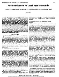
Figure 1: Embedded time Markov chain describing the state of a saturated station’s back-off counter (s(t), b(t))

Based on the definition of the 802.11 DCF in Section 2, the system of pairs (s(t), b(t)) for all stations clearly forms an aperiodic, irreducible Markov chain. The main difficulty in analyzing its characteristics is that the state-space grows exponentially with the number of stations in the WLAN, n. Bianchi’s [6] solution to this modeling difficulty was to decouple stations through the following approximation. For a station i ∈ {1, . . . , n} in the WLAN, define Ck := 1 if the k th transmission by station i results in a collision and Ck := 0 if it results in a success. Assumption 1 (Bianchi’s Decoupling Approximation) For each station i ∈ {1, . . . , n}, the collision sequence {Ck } is i.i.d. with P (Ck = 1) = pi . This assumption says that for each station i, conditioned on that station attempting transmission (i.e. b(t) = 0), there is a fixed probability pi that it experiences a collision irrespective of its past experience. In particular, station i’s conditional collision probability, pi , is assumed to be independent of the station’s back-off stage s(t). Omitting the station label i, the aperiodic Markov chain describing the evolution of (s(t), b(t)) is depicted in Figure 1, assuming that the conditional collision probability p is known. We are interested in the stationary probability that the station is attempting transmission, τ (p),

7 given the conditional collision probability is p: τ (p) =

M X

π(j, 0),

j=0

where π(i, j) is the stationary distribution of the Markov chain. With a little elementary algebra, π(i, j) can be determined explicitly [7]. Providing more insight, as observed independently by Kumar, Altman, Miorandi and Goyal [32][33] and Bianchi and Tinnirello [8], τ (p) can be identified directly as a deduction from the renewal reward theorem. Let Uj denote the uniform distribution on {1, . . . , Wj }, so that this variable counts how many idle slots a station observes before transmission rather than its back-off counter. Then we have that E(1 + C0 + C0 C1 + · · · + C0 · · · CM ) E(U0 + C0 U1 + C0 C1 U2 + · · · + C0 · · · CM UM ) 1 + p + p2 + · · · + pM , = W0 /2 + pW1 /2 + · · · + pM WM /2

τ (p) =

(1)

where the renewal epoch is the number of idle slots a packet spends being processed in the MAC and the reward is the number of attempted transmissions during an epoch. The use of the renewal reward theorem makes it clear that the decoupled model is insensitive to the back-off distribution at any given back-off stage. The uniform distributions {Uj } only enter into the formula in equation (1) through their expectation, so that - for example - any other collection of back-off distributions with the same mean number of slots to be counted down, Wj /2, at each stage, j, will give rise to the same stationary attempt probability τ (p). For 802.11-like parameters, with Wj = 2min(j,m) W0 for j ∈ {0, . . . , M }, equation (1) gives τ (p) =

2(1 − pM +1 ) , W0 (1 − p − p(2p)m )/(1 − 2p) − W0 2m pM +1

(2)

where the case of p = 1/2 is obtained by taking the limit p → 1/2. For 802.11b with W0 = 32, m = 5 and M = 11, τ (p) defined in equation (2) is plotted in Figure 2 as a function of p. The self-consistent equation in this mean field model then arises after assuming that every station in the WLAN is small relative to the entire WLAN. With this in mind, observe that the probability a station does not experience a collision given it is attempting transmission is the probability that no other station is transmitting: 1 − p = (1 − τ (p))n−1 .

(3)

As τ (p) defined for 802.11b in equation (2) is a strictly monotone decreasing function on [0, 1], there is a unique solution, p∗ , of the fixed point equation (3). This solution can be readily found numerically and p∗ is interpreted as the “real” collision probability for a station in the WLAN.

8 0.07

Stationary Transmission Probability tau(p)

0.06

0.05

0.04

0.03

0.02

0.01

0

0

0.2

0.4 0.6 Conditional Collision Probability p

0.8

1

Figure 2: Stationary transmission probability τ (p) as a function of the conditional collision probability p for the IEEE 802.11b parameterization

Armed with p∗ and τ ∗ := τ (p∗ ), we are now in a position to determine performance metrics. For simplicity, assume that idle slots are of real-time length σ and that all transmissions take time T on the medium regardless of whether they correspond to a collision or a successful transmission. The latter is not true in practice, but the distinction in times between collisions and successful transmissions can be readily incorporated if necessary. Let R denote the physical layer transmission rate in Mbps. As a consequence of ergodicity, the long run throughput, S, of each station can be determined, almost surely, from the stationary probabilities τ ∗ and p∗ : S=

τ ∗ (1 − τ ∗ )n−1 T R τ ∗ (1 − p∗ )T R = , (1 − τ ∗ )(1 − p∗ )σ + (1 − (1 − τ ∗ )(1 − p∗ ))T (1 − τ ∗ )n σ + (1 − (1 − τ ∗ )n )T

(4)

where the numerator is the stationary probability of successful transmission times the amount of data sent per transmission and the denominator is stationary average real time between counter decrements. Throughput predictions from Bianchi’s model are remarkably accurate. For example, Figure 3∗ plots measured throughput from a real test-bed WLAN as well as the model’s predictions. Lines are used for the theoretical predictions, as otherwise one cannot distinguish the theory from experiment. If one believes that the decoupling approximation, Assumption 1, is reasonable, then one could plausibly expect the model to be good for large n. However, note that the model is exact when n = 1 as the self-consistent equation (3) gives p = 0. Even for n = 2, which one ∗

The data used to generate this figure was donated by Malone, Dangerfield and Leith [38].

9 2

Measured Model

1.8

S, per-station throughput (Mbps)

1.6 1.4 1.2 1 0.8 0.6 0.4 0.2 0

2

4

6

8 n, number of stations

10

12

14

Figure 3: Measured and predicted throughput per station in a WLAN consisting of n stations using the 802.11 DCF and the 802.11b 11Mbps physical rate – data from [38]

might believe to be the worst case for the approximation, predictions are precise. Thus, due to the intuitive appeal of the model’s structure, as well as its predictive success, Bianchi’s basic paradigm has been widely adopted for models that expand on its original range of applicability, which is something we shall return to in Section 4.

3.2

On the appropriateness of the decoupling approximation

The fundamental decoupling hypothesis in Bianchi’s approach is that collisions form an i.i.d process for each station. As the primary aim of increasing the contention window after a collision is to reduce the likelihood of repeated collisions, one might suspect that this ansatz is dubious. One way to provide support for this approximation is to perform an asymptotic analysis of the fully-coupled system as the number of stations in the WLAN tends to infinity. Independently of each other and using distinct methodologies, Bordenave, McDonald and Proutière [9][11] and Sharma, Ganesh and Key [44][45], followed by further analysis by Vvedenskaya and Suhov [52], studied similar models in asymptotic limiting regimes† . One aim of these papers is to provide a theoretical justification of the decoupling approximation, Assumption 1. These authors study the full system described by the 802.11 DCF, albeit with the following simplifying approximation that is distinct from Assumption 1. † Benaim and Le Boudec [4] have also introduced a general mean field model that touches upon the veracity of Bianchi’s throughput formula.

10 Assumption 2 (Full System Analysis Approximation) At each back-off stage j, the back-off counter is chosen from a geometric distribution with mean (Wj − 1)/2. The mean of the geometric distribution is chosen to match the mean of the uniform distribution in the 802.11 DCF protocol. Both sets of authors state that they believe that this assumption is not crucial to their arguments, but it does simplify the analysis. In particular, in the notation of [44][45], in a WLAN with n identically parameterized stations, a natural description of the system is the vector +1 X n (t) = (Xn0 (t), . . . , XnM (t)) ∈ ZM +

(5)

denoting the number of stations in each of the back-off stages 0 through M . With Assumption 2 in force, the process (5) is Markovian; without Assumption 2, in addition one would need to record the back-off counter of each station. In order to obtain a meaningful limit, the natural fluid scaling is to look at sample path of the fraction of stations in each back-off stage 1 X n ([nt]), where [t] is the integer part of t, n and to reduce the access probability at each back-off stage with the number of stations in the WLAN by scaling up the contention window, nWj . Let us first make a few definitions so that we can state one of the main results of Sharma et +1 al. before turning to the results of Bordenave et al. Let x = (x0 , . . . , xM ) ∈ ZM be such + PM PM that j=0 xj = n and define ||x|| := j=0 |xj |. The conditional expected change in the state of the WLAN consisting of n stations given that the system is currently in state x is f (n) (x) := E (X n (t + 1) − X n (t)|X n (t) = x) . The following functional law of large numbers appears as [45, Theorem 5]. Theorem 1 (Sharma, Ganesh & Key) For every t > 0, 1 lim sup X n ([nt]) − Y (t) = 0 almost surely, n→∞ 0≤s≤t n where Y (t) is the unique solution of the differential equation dY (t) = F (Y (t)) dt

(6)

and F (x) = limn→∞ f (n) (nx). The method of proof employed is relatively direct. It follows primarily through astute bounds on the stationary probability that the medium is observed idle and the development of uniform

11 bounds to show that F (x) is Lipschitz. In addition to this result, inter alia, the authors prove that the equation F (x) = 0 has a unique solution and that if M = 1 then the differential equation (6) converges to a unique equilibrium point satisfying F (y) = 0 from all possible initial states [45, Proposition 3]. Simulation evidence is presented to support a conjecture that this holds true also for M > 1. Vvedenskaya and Suhov [52] raise the possibility of the existence of metastable solutions in this model with [52, Theorem 2] providing a simple methodology to determine how many solutions exist. They also provide an example where {E(Uj )} is not a monotone decreasing sequence and metastability appears. The Poisson approximation analysis of the Sharma et al. model by Vvedenskaya and Suhov [52] reveals that in this limit the number of stations that transmit in a given slot is a Poisson random variable. In particular, this is true with an unchanged Poisson rate if we tag any finite collection of stations and condition on them being in given back-off stages. Thus this fluid limit analysis of the fully coupled model provides evidence that the decoupling Assumption 1 holds for any given finite sub-collection of stations in the WLAN during a transient time interval. The independent, and practically simultaneous, analysis of a similar model performed by Bordenave, McDonald and Proutière employs, arguably, more sophisticated tools. It is based on the notion of propagation of chaos due to Mark Kac, where the marginals of a coupled system that is started appropriately are almost independent in the limit as the system becomes large. In particular, the authors use a method developed by Sznitman [48] and extended by Graham [22]. We require a few definitions to describe two of their main results. The state of the system is the vector of back-off stages of each of the n stations at each embedded time, (s1 (t), . . . , sn (t)). Because of Assumption 2, the individual back-off values need not be recorded as part of the system state. Note that the state-space is growing as a function of the number of stations in the WLAN, n. As with Sharma et al., the attempt probabilities are scaled down by scaling up the window size linearly with n to nWj . The scaling employed for the state vector is (n)

si (t) := si ([nt]), where the time rescaling corrects for the fact that the expected time between attempted transmissions for each station is decreasing linearly in n. Let D denote the space rightcontinuous functions having left-hand limits over R+ taking values in the set of possible back-off stages, {0, . . . , M }, equipped with the Skorohod (J1 ) topology [47]. Let P(X ) denote the set of probability measures on a set X . The following is a sub-result of the more general [9, Theorem 1]. Theorem 2 (Bordenave, McDonald and Prouti` ere) Assume that the initial values si (0), i = 1, . . . , n, are exchangeable and that the system is initially chaotic. That is, that there exists Y (0) ∈ P({0, . . . , M }) such that the sequence of random variables X n (0)/n (where

12 X n (t) is defined in equation (5)) converges weakly to δY (0) when n → ∞. Or, equivalently‡ , with L denoting the law of the process, that (n)

lim L(si (0), i ∈ I) = Y (0)⊗|I|

weakly in P({0, . . . , M }|I| )

n→∞

for all finite subsets I ⊂ N \ {0}. Then we have propagation of chaos: there exists Y ∈ P(D) such that the sequence of random variables X n ([nt])/n converge weakly to δY or, equivalently, that for all finite subsets I ⊂ N \ {0}, (n)

lim L(si (·), i ∈ I) = Y ⊗|I|

n→∞

weakly in P(D|I| ).

Furthermore the marginals of Y satisfy dY = F (Y (t)), dt as in equation (6). Due to the topologies employed, both Theorem 1 and Theorem 2 are results solely concerned with compact time intervals. In order to justify Bianchi’s decoupling assumption in terms of stationary behavior one requires a result in the stationary, rather than the transient, regime. Having identified the dynamical system describing the evolution of the empirical measure, assuming it is globally stable§ , this is the subject of the following theorem of Bordenave, McDonald and Proutière [9, Theorem 4]. Theorem 3 (Bordenave, McDonald and Prouti` ere) In equilibrium, for all subsets I ∈ N of finite cardinality |I|, (n)

⊗|I|

lim Lst ((si (·))i∈I ) = Yst

n→∞

weakly in P(D|I| ),

where the subscript st indicates the stationary behavior of the system. Modulo a rigorous justification that replacing uniform distributions with geometric distributions in Assumption 2 has no bearing on the deductions, in this limiting regime these results support Bianchi’s decoupling assumption Assumption 1. That does not mean, however, that there are no more interesting questions to be addressed within this asymptotic model. The following open problem was proposed by Charles Bordenave¶ : in a WLAN of n stations, let Nn (t) count the total number of packets successfully transmitted by all stations prior to ‡

The equivalence is due to Sznitman [48]. See [11, §5] for more on global stability of the empirical measure dynamical system. ¶ Private communication. §

13 Saturated

0.05

0.35 0.3

0.03 Collision Probability

AutoCovariance Coefficient

0.04

0.02 0.01 0

0.25 0.2 0.15 Bianchi N=2 NS N=2 Bianchi N=5 NS N=5 Bianchi N=10 NS N=10

0.1

−0.01 −0.02

Saturated

0.4 N=2 N=5 N=10

0.05

0

5

10 Lag

15

20

0 −1

0

1

2

3

4

5 6 7 Backoff Stage

8

9

10

11

12

Figure 4: Normalized auto-covariances and empirical collision probabilities as a function of back-off stage for a simulated collision sequence, C1 , . . . , CK – data from [26]

time t. What is the appropriate scaling tn such that the random variable Nn (tn )/n converges to a non-trivial distribution and what are the characteristics of this distribution? Moreover, in the following section we state results of Ramaiyan, Kumar and Altman [42] regarding Bianchi’s decoupled model that show that for appropriately chosen contention window size sequence, {Wj }, metastable states can exist. It would be interesting to know if this metastability translates to metastability in the fluid limit model. Before we leave this section, we note that it is possible to check the veracity of Assumption 1 from a statistical perspective by testing long sequences C1 , . . . , CK recorded from either simulation or experiment in conjunction with the back-off stage at which each transmission took place. This is the procedure pursued by Huang et al. [26][25]. For the saturated WLAN, this work supports Assumption 1, even though the approximation is not precisely true. Figure 4 was created with data from [26]. It reports on the empirically observed auto-covariances for C1 , . . . , CK from a station in a WLAN consisting of N stations. Assuming that the sequence {Ck } is wide sense stationary, it supports the independence hypothesis. To check for identical distributions, Figure 4 also reports a scatter-plot for all stations in the WLAN of the maximum likelihood estimator for collision probabilities conditioned on the station being in a particular back-off stage. This plot shows some structure, where the likelihood of collision at the first back-off stage is lower than at the zeroth back-off stage, which is a reasonable consequence of the doubling of the back-off window. Collision probabilities then rise as a function of back-off stage, presumably as selecting from a large back-off window results in the system being in statistical equilibrium by the next attempted transmission. For reference, the predicted collision probability from Bianchi’s model is also plotted.

14

3.3

On the nature of solutions of the self-consistent equations

For a saturated WLAN with 802.11 DCF parameters, it is clear that the fixed point equation (3) in Bianchi’s model admits only a single solution. Is this sufficient to ensure that the solution of that equation determines the equilibrium of the decoupled system? No, is the obvious (and correct) answer. In the decoupled model, we should at least be looking at solutions of the system of n equations Y (1 − τ (pj )) for i ∈ {1, . . . , n}. (7) 1 − pi = j6=i

That is, we should not restrict ourselves solely to considering symmetric solutions. In [42] Ramaiyan, Kumar and Altman investigate the fixed point equations (7) in detail. Ruining the surprise somewhat, they show that for the 802.11 DCF parameterization, the equations (7) admit only a symmetric solution (see the remark after [42, Theorem 5.2]). That is, the unique solution to (7) is (p1 , . . . , pn ) = (p, . . . , p), where p is the solution to equation (3). However, they do provide examples of back-off window mean sequences {E(Uj )} where this is not the case and the equations (7) admit non-symmetric solutions. As all stations are parameterized in the same way, this gives rise to metastability (which the authors call multistable solutions) and predictions based on a symmetric solution to (3) do not agree with results from simulation. Instead the simulated observations correspond to time-averages of the metastable solutions. Here we summarize some of their deductions and highlight questions raised in relation to the analysis in Section 3.2. The following result, [42, Theorem 5.1], which first appeared in [33], provides a sufficient condition for the uniqueness of a symmetric solution. Theorem 4 (Kumar, Altman, Miorandi & Goyal) If {E(Uj ) : j = 0, . . . , n} is a nondecreasing sequence (so that τ (p) is non-increasing), then the symmetric fixed point equation (3) admits a unique solution. Let us rewrite the full equations (3) as a vector equation in [0, 1]n : p = Γ(T(p)),

(8)

where, for x ∈ [0, 1]n ,  T(x) = (τ (x1 ), . . . , τ (xn )) and Γ(x) = 1 −

 Y j6=1

(1 − xj ), . . . , 1 −

Y

(1 − xj ) .

j6=n

As both T and Γ are continuous functions, by Brouwer’s fixed point theorem, there is at least one fixed point of the equation (8).

15 In [42] a sufficient (though not necessary) condition for a unique solution of the vector fixed point equation (8) to exist and be symmetric, is developed in terms of the probability that the medium is observed idle. Note that for any p = (p1 , . . . , pn ) that is a solution to the fixed point equation (8), the quantity I(pi ) = (1 − pi )(1 − τ (pi )) =

n Y Y (1 − τ (pj ))(1 − τ (pi )) = (1 − τ (pj )) j6=i

j=1

is the same for all i. Physically, this lack of dependence on i is because I(pi ) corresponds to the probability that station i observes that the medium is idle. As all stations are continuously observing the same medium, this is the same for all stations. Ramaiyan et al. establish that if I(p) is one-to-one, then there is a unique symmetric fixed point, [42, remark after Theorem 5.2]. Regarding stationary attempt probabilities that arise from 802.11-like parameters, the following appears as [42, Theorem 5.2]. Theorem 5 (Ramaiyan, Kumar & Altman) If M ≥ 1, κ ≥ 2, E(U0 ) > 2κ+1, E(Uj ) = κmin(j,m) E(U0 ) for j = 1, . . . , M , then the vector fixed point equation (8) admits a unique solution p1 = (p, . . . , p), where p is the solution to the symmetric fixed point equation (3). This result applies to 802.11b where M = 11, κ = 2 and E(U0 ) = 16. Theorem 5 provides sufficient conditions for the existence of a unique solution, but the authors also provide examples where these sufficient conditions do not hold and metastability is observed in simulation and through the numerical solution of the equation (8). Consider a WLAN consisting of n stations with the following parameterizations. Example 1: n = 10, m = 4, M = ∞, E(Uj ) = 1 for j = 0, . . . , 4, E(Uj ) = 64 for j = 5, . . .. Example 2: n = 20, m = 7, M = 7, E(Uj ) = 3j for j = 0, . . . , 7. Neither of these examples satisfy the conditions of Theorem 5 and both exhibit metastability. The reason can be readily understood: in both cases, for long periods of time the system settles into a situation where some stations can frequently transmit successfully, while others repeatedly experience collisions with a large number of idle slots between their attempted transmissions. As all stations have the same parameters, the system has a natural symmetry where the number of stations in each group is unchanging, but their constituent members revolve. This is easier to see in the former example, where only a single station can be in back-off stage 0 at any one time. The second example is presented for its appeal as appearing similar to the parameterization of the 802.11b/a/g protocols, the important difference being the small value of E(U0 ) in the example. A consequence of this metastability is that the solution of the symmetric equations (3) gives inaccurate predictions and the system possesses short-term unfairness. It would be interesting

16 to know if scaled versions of these examples, within the models described in Section 3.2, exhibit metastability and if the fluid limit models can shed more light on necessary and sufficient conditions for metastability. This sort of metastability, which arises despite {E(Uj )} being a monotone decreasing sequence, may only be visible in the system state of Bordenave et al. as individual stations are not distinguishable in the Sharma et al. system state. The metastability example presented in [52] is based on a non-monotone decreasing sequence {E(Uj )}.

4

Non-saturated WLANs

A running assumption so far has been that all stations are saturated, so that they always have packets to transmit. The motivation for this condition is to determine the long-run stable maximum throughput of the system. It has the added benefit that it simplifies analysis as queueing dynamics can be ignored. However, traffic is typically bursty in nature, so that most operational WLANs are not saturated. For example, voice conversations are typically low-rate, transmitting small packets during speech and transmitting nothing during silence periods. The International Telecommunications Union (ITU) standard that dictates the stochastic model to be used for performance evaluation of conversation speech, ITU-T P.59 [51], is a three state Markov Additive Process. It is evident from the parameterization of this model that there are long silent periods from both sources of traffic. As Bianchi’s modeling paradigm demonstrated its value for saturated WLANs, there is a large collection of published articles in the telecommunications literature that extends it to the non-saturated setting. A selection of this work is [1, 21, 53, 12, 27, 17, 41, 39, 15, 54, 24] The practical aim of these papers is to understand how the 802.11 DCF shares bandwidth as a function of traffic load and its consequent impact on fairness. Looking forward to the 802.11e EDCA, these models are also used to understand how setting distinct MAC parameters for different stations can enable prioritization. As far as we are aware, unlike the results reported in Sections 3.2 and 3.3 for saturated WLANs, there has been no formal justification of this extension of the paradigm to nonsaturated WLANs, although these models are reported to make accurate predictions. We would like to explore the implications of this fact and the additional complications that arise due to the introduction of finite load traffic sources. The primary difficulty to modeling non-saturated stations comes from the fact that the service process in Bianchi’s model runs in embedded time. For example, consider a station as a node in a queueing system. Packet arrivals are naturally described in real-time (packets per second), whereas the service process as dictated by the 802.11b DCF runs in embedded time based on idle slots on the medium.

17 Unsaturated, BIg Buffer

0.14

N=2 λ=200 N=5 λ=80 N=10 λ=40

0.12

Collision Probability

0.1 0.08 0.06 0.04 0.02 0 −1

0

1

2

3

4 5 6 Backoff Stage

7

8

9

10

11

Figure 5: Empirical collision probabilities as a function of back-off stage for a non-saturated collision sequence, C1 , . . . , CK – data from [26]

Let us develop a non-saturated model along the lines of the work referenced above, from which the main issues should become apparent. Our starting point is Bianchi’s decoupling approximation, Assumption 1. Before moving on to highlight further issues, we note that the appropriateness of this assumption is already in doubt. For a simulated non-saturated system with where each station’s buffer is infinite, Figure 5, created with data from [26], shows the maximum likelihood estimator for collision probabilities conditioned on the station being in a particular back-off stage. There is clear structure in the graph where the collision probability at the first back-off stage is higher than at the zeroth. This is readily understood: in a lightly loaded system, for long periods only a single station has a packet to send and thus it doesn’t often experience collisions at back-off stage zero. Conditioning on a station experiencing a collision at the first back-off stage is closely related to conditioning on at least one other station having a packet to transmit at that time, hence the increase in collision probability. It would be interesting to know if this feature persists in the fluid limit. Comparing this figure with the saturated equivalent, Figure 4, reveals that the relative fluctuations in the present graph are larger than in the former. Returning to the model, let us initially work in embedded time and start with a small modification to the Markov chain depicted in Figure 1. Ignoring post-back-off (mentioned in Section 2) by assuming all packets experience a back-off period, let us add a single additional state, labeled (−1, 0), corresponding to the station having no packets awaiting transmission. We introduce two new probabilities that we will ultimately relate to the offered traffic load: the probability a packet arrives to the MAC during an average slot time on the medium, r, and the probability that after a successful transmission a packet is buffered and available to the MAC, q. For a given station, define the following sequence: let Qk = 1 if after the k th successful transmission (or packet discard due to retry limit exceedance) there is a packet

18 1−r r

−1,0

(1−p)q (1−p)(1−q)

1

0,0

1

0,1

1

1

0,2

0,W−1 0

p

(1−p)q (1−p)(1−q)

1

1,0

1

1,1

1

1

1,2

1,W−1 1

p

(1−p)q (1−p)(1−q)

1

m,0

1

m,1

1

1

m,2

m,W−1 m

p

q 1−q

1

M,0

1

M,1

1

M,2

1

M,W−1 m

Figure 6: Embedded time Markov chain describing the state of a non-saturated station’s back-off counter (s(t), b(t))

waiting for service and Qk = 0 if there is no packet in the station’s queue. We make the following assumption, which is widely used in the literature, albeit often implicitly. Assumption 3 (Decoupled Queueing) For each station i, the sequence {Qk } is i.i.d. with P (Q = 1) = qi . Omitting the station label i, after each successful transmission or packet-discard, an independent Bernoulli queue-busy random variable, Q with P (Q = 1) = q and P (Q = 0) = 1 − q, is observed. If Q = 1, then the station’s queue has at least one packet awaiting transmission and a new back-off counter is selected. If Q = 0, there is no packet awaiting transmission and the station remains idle between each counter decrement with probability 1 − r. These transitions are graphically represented in Figure 6. We are not aware of the application of the renewal reward theorem to determine the stationary probability that a station is attempting transmission in the non-saturated modeling literature, but it can be used exactly as in the saturated case and provides the quickest mechanism for determining the stationary probability that a station is attempting transmission. Note that after a transmission (or packet discard), the expected number of slots until another packet is available for transmission is the probability that there is no packet awaiting transmission,

19 1 − q, times the expected number of slots until a packet arrives, 1/r, so that: E(1 + C0 + C0 C1 + · · · + C0 · · · CM ) E(U0 + C0 U1 + C0 C1 U2 + · · · + C0 · · · CM UM ) + (1 − q)/r 1 + p + p2 + · · · + pM = , W0 /2 + pW1 /2 + · · · + pM WM /2 + (1 − q)/r

τ (p, q, r) =

(9)

where the renewal epoch is the time between the MAC’s initiation of service on consecutive packets. Note that in the non-saturated case the use of the renewal reward theorem still demonstrates that the only impact on the stationary attempt probability of the back-off distributions is through their expected value. With Wj = 2min(j,m) W0 for j ∈ {0, . . . , M }, as in the 802.11 parameterization, we have that τ (p, q, r) =

2(1 − pM +1 ) . W0 (1 − p − p(2p)m )/(1 − 2p) − W0 2m pM +1 + (1 − q)/r

In order to obtain value from this model, it is necessary to relate the embedded time load parameters r and q to the real-time offered load in packets per second. As with most authors, we restrict our attention to Poisson arrival processes. Assumption 4 (Poisson Arrivals) Station i’s packet arrivals are Poisson at rate λi . Label the expected time between counter decrements as n Y E(D) = (1 − τi (pi ))σ + i=1

! n Y 1 − (1 − τi (pi )) T, i=1

and the expected number of counter decrements from when a packet starts being processed by the MAC until its successful transmission (or it is discarded) to be E(B) =

W0 (1 − p − p(2p)m ) W0 2m pM +1 − 2(1 − 2p)(1 − p) 2(1 − p)

for the 802.11-like parameterization. Case 1: no buffer. In the absence of buffering, the natural approximations to use are q = 0 and 1 − r = exp(−λE(D)). That is, as there is no buffering beyond the packet in the MAC, no packets can be awaiting processing at the end of a service period and the likelihood of not seeing a packet arrival during a slot of average length is the probability that an inter-arrival time is longer the average slot length. The latter is clearly an approximation, albeit a widely adopted one, as it does not take into account variability in real-time length of slots. With this caveat, Assumption 3 requires no further defence.

20 Case 2: infinite buffer. In this case the station is effectively an M/G/1 queue, e.g. [2]. Here we use a common approximation: we assume that after a packet is serviced, the probability that the queue is busy can be approximated by the stationary probability that the corresponding M/G/1 queue has content in its buffer. That is, from standard results in queueing theory it follows that q = min(1, λE(B)E(D)). As in the no buffer case, we still use the approximation that 1 − r = exp(−λE(D)), so that we have q = min(1, −E(B) log(1 − r))). In both the no buffer and infinite buffer cases the function τ (p, q, r) is reduced to a function of two variables τ (p, r): p the probability of collision conditioned on an attempted transmission and the load parameter r which is related to the real-time arrival rate λ through λ = − log(1− r)/E(D). An inverse method is typically employed to solve models of this sort. One selects r ∈ [0, 1]n and identifies the solution to the fixed point equations: Y 1 − pi = (1 − τ (pj , rj )) for i = 1, . . . , n. (10) j6=i

Once the solution, p∗ , has been determined, one determines what real-time load corresponded to r is by evaluating E(D) and then λ. Let us consider each of the apparent challenges to rigor that are implicit in this approach. Firstly, we are assuming that for each r that there is a unique solution p∗ to (10). Although not intended for this purpose, a result of Ramaiyan, Kumar and Altman [42] provides a sufficient condition for this to be true. With a change of notation, [42, Theorem 5.3] proves the following. Theorem 6 (Ramaiyan, Kumar & Altman) Assume r is given. For all i ∈ {1, . . . , n}, if the attempt probability τ (p, ri ) is a decreasing function of p and (1 − p)(1 − τ (p, ri )) is a strictly monotone function on [0, 1], then the system of equations (10) has a unique fixed point p∗ . Secondly, in the infinite buffer model, the probability that a station’s queue is busy after each transmission is assumed to form an i.i.d. sequence. This is a dubious approximation. Even if a station’s queue-busy sequence {Qk } constituted independent random variables, clearly the queue-busy probability, P (Q = 1) = q depends upon back-off stage. Higher back-off stages correspond to longer MAC service times, which in turn lead to a significantly higher likelihood of a packet arrival to the queue. The fallaciousness of this assumption is demonstrated empirically in Huang et al. [26][25]. However, we note that despite this difficulty with the model’s fundamental assumptions, models based on it appear to make good throughput predictions and that this conundrum is partially resolved in [24]. In our discussion here we will treat the system as a model and not fret further about the veracity of its assumptions.

21 The third and final point of concern is that we are implicitly hoping that the mapping from the embedded time load parameter to the real-time load parameter, r 7→ λ, is one-to-one. We will demonstrate that this is not true in general and relate it to a conjecture about the queue stability region in the decoupled model; a conjecture that we do not believe has been highlighted before in the literature. This lack of one-to-oneness in the map r 7→ λ is, we suggest, related to identifying the stability region of the queueing system. That is, in identifying the set of arrival rates λ for which the queues at all stations are stable. Note that for stations sharing a communications channel by use of random access protocol, identifying stability regions in a non-decoupled system is a non-trivial task (e.g. H˚ astad, Leighton and Rogoff [23], Ephremides and Hajek [20] and Bordenave, McDonald and Proutière [10]). Let us demonstrate this feature here for a symmetrically loaded network, r = r1 and λ = λ1, with the model we have introduced. Consider a WLAN consisting of n = 10 symmetrically loaded stations all of which transmit 560 byte packets at R = 11Mbps and have the same parameters: W0 = 32, m = 5 and M = ∞ so that the station normalized throughput is:  1  , if λ ≤ λT R E(B)E(D) S= TR 1   if λ > , E(B)E(D) E(B)E(D) That is, as the station has an infinite buffer, throughput is the arrival rate so long as the arrival rate is less than the service rate and otherwise it is the service rate. Having solved for a symmetric solution p∗ to the fixed point equations (10), Figure 7 plots the real-time offered load λ as a function of the internal offered load parameter r. This figure shows a range where three distinct r values give rise to the same λ. Figure 8 reveals how this impacts on throughput predictions: there are two potential throughputs at certain offered loads. We conjecture that where multiple solutions exist, even if r 6= r1, it is the lowest throughput that corresponds to the stable solution. This conjecture is supported by simulation and experimental evidence, but has not been proven rigorously. To explain why a triple of r values giving rise to a single λ, we return to the no-buffer model where q = 0. Solving for the same system, but with stations having no buffers, Figure 9 plots λ versus r and per-station throughput, as determined from equation (4), versus λ. There is clearly a one-to-one relationship between r and λ, but throughput is not a monotonic function of λ. This pre-saturation throughput peak is a well-known property of stochastic MAC protocols (e.g. Bertsekas and Gallager [5]). In the decoupled model, as τ (p, r) is a continuous function of r that covers the same range for both the no buffer and infinite buffer models, the throughput graphs must cover the same range of values. In the infinite buffer case, this pre-saturation throughput peak appears to occur as a temporary unstable solution of the system. While this argument supports the conjecture that where multiple solutions exist it is the lowest throughput that corresponds to the stable solution and that the other two are transient, a rigorous proof is lacking.

22

10 Symmetric Non-saturated Stations


0.055

0.0355

0.05 0.045

0.035

0.035

Arrival Rate Lambda

Arrival Rate Lambda

0.04

0.03 0.025 0.02

0.0345

0.034

0.015 0.0335

0.01 0.005 0

0

0.005

0.01

0.015

0.02

0.025

0.03

0.035

0.033

0.04

0.01

0.012

Embedded Arrival Probability r

0.014

0.016

0.018

0.02

0.022

0.024

0.026

0.028


Figure 7: Real-time arrival rate, λ, versus embedded packet arrival probability, r, in a symmetric system of n = 10 stations with infinite buffers; second graph is a closeup of the first graph revealing lack of one-to-one relationship



0.39

0.385

0.38 0.38 Throughput per Station (Mbps)

Throughput per Station (Mbps)

0.37 0.36 0.35 0.34 0.33 0.32

0.375

0.37

0.365

0.31 0.3

0.3

0.35

0.4 Arrival Rate (Mbps)

0.45

0.5

0.36 0.36

0.365

0.37 0.375 Arrival Rate (Mbps)

0.38

0.385

Figure 8: Per-station throughput versus real-time arrival rate, λ, for a symmetric system of n = 10 stations with infinite buffers; second graph is a closeup of the first graph revealing two possible throughputs for some values of λ

23 10 Symmetric Non-saturated Stations


0.08

0.4

0.07 0.38

Throughput per Station (Mbps)

Arrival Rate Lambda

0.06

0.05

0.04

0.03

0.36

0.34

0.32

0.02 0.3 0.01

0

0

0.005

0.01

0.015

0.02

0.025


0.03

0.035

0.04

0.28

0.4

0.6

0.8

1

1.2

1.4

1.6

1.8

2

Arrival Rate (Mbps)

Figure 9: Symmetric system of n = 10 stations with no buffers. Real-time arrival rate, λ, versus embedded packet arrival probability, r, and per-station throughput versus λ

5

Mesh networks

All discussion so far has considered a single WLAN; a collection of n stations all in the same physical space wishing to communicate via a single shared wireless resource. One of the practically important uses of 802.11 technology is to facilitate mesh networks where, as well as communicating directly with their neighbors in the WLAN, stations communicate with more distant stations in another WLAN by having their messages relayed by 802.11 equipped intermediaries called mesh points. Mesh points are members of more than one single WLAN and can relay traffic between the WLANs of which they are members. Mesh networking is the subject of the 802.11s standard, which is likely to be ratified in late 2009. It still employs the 802.11b DCF MAC or its more sophisticated variant the 802.11 EDCA, but standardizes packet-forwarding rules. Mesh networking poses problems for both theory and practice. The primary practical issue is the interaction of stations using the same frequency at distances such that they can interfere, but not communicate with each other. This difficulty leads to the hidden and exposed node problems. We shall not consider these problems further here as there is an engineering solution that is employed to overcome them. There are three non-interfering frequencies available in 802.11b/g and twelve in 802.11a. WLANs operating on these frequencies can be in the same physical space without interfering with each other. A practical solution to the hidden/exposed node problem in wireless mesh networking is to equip mesh points with more than one radio. Each radio operates on a non-interfering frequency, so that the forwarding station can relay data between two WLANs without leading to hidden or exposed nodes in either. Note that non-saturated models are a necessary pre-cursor to modeling mesh networks as even if initial stations are saturated, stations relaying traffic may not be. As an aside, enabling distinct WLANs to select their

24 operating frequency without direct communication leads to a problem that can be posed as a decentralized graph colouring problem, e.g. [35][30][18]. Mesh networking is the subject of extensive mathematical analysis, worthy of a review in and of itself, but here we focus solely on a approach in spirit of Bianchi’s original work. A decoupled model for multi-radio mesh networks in the absence of hidden and exposed nodes is proposed in [16]. The primary difficulty in modeling this system is that the embedded time in each individual WLAN (collection of stations that are all operating on the same frequency and are sharing the same embedded time channel) in the mesh network is running at a different real-time speed. WLANs in the mesh that have a small number stations will see many idle slots and thus run quickly, while the opposite is true for WLANs in which there is a lot of contention for the medium. The primary idea in [16] is to model each WLAN with an a priori assumed input of traffic from the mesh. Solving the appropriate fixed point equations, one can then predict the throughput for each station in the WLAN. If some of the WLAN’s traffic will be relayed through other parts of the mesh, the WLAN’s throughput corresponds to its rate of departures and this becomes the input to another WLAN in the mesh. Assuming the departures are Poisson, which is reasonable if the original input is Poisson and the WLANs are not heavily loaded [26][25], one is then looking for a solution to the entire coupled system that correctly balances the arrival and departure rates for relayed traffic throughout the mesh. It requires a large volume of tedious notation to explicitly write down the equations to be solved. This can be found in [16], where examples are presented that illustrate this approach can make good predictions of the overall network behavior. Nothing has been proven formally about this model with regards either the appropriateness of the decoupling approximation or the nature of the solutions of this substantially more complex set of self-consistent equations. As mesh networks form one of the most exciting applications of 802.11 technology, any results in this direction would be likely to be of interest to telecommunications community.

6

Summary and Discussion

Let us enumerate the questions that have arisen. 1. §3 For saturated WLANs with appropriately chosen back-off window sizes, metastability is observed in the decoupled model. Does this metastability also appear in the fullycoupled fluid limit model? If so, can the fluid limit model shed more light on the phenomenon? 2. §3 In the coupled WLAN model with n stations, let Nn (t) count the total number of packets successfully transmitted by all stations prior to time t. What is the appropriate scaling tn such that the random variable Nn (tn )/n converges to a non-trivial distribution

25 and what are the characteristics of this distribution?k 3. §4 If a WLAN is non-saturated, is the decoupling approximation appropriate and, if so, can a fluid limit analysis of a coupled model support it?∗∗ 4. §4 Consider the non-saturated decoupled model with infinite buffers. The relationship between the load in embedded time, r, to the real-time Poisson offered load, λ, is not one-to-one. Can it be shown that there is a unique stable solution at all real offered loads that corresponds to the long-run behavior of the system? If so, does this give insight into the identification of the stability region of the fully coupled model, which is known to be difficult to analyse? 5. §4 Driven by Markovian convenience, all of the decoupled finite load models that we cite assume that packet arrivals follow a Poisson process. In the presence of infinite buffers and without MAC-level packet discard (i.e. M = ∞), can this assumption be relaxed to more general arrivals processes without changing the stability region for the decoupled models?†† 6. §5 For the decoupled, non-saturated, mesh model, what can be said about the existence and uniqueness of a solution to the global fixed point equation? Can metastable solutions exist in mesh networks for parameterizations that would not give rise to them in WLANs? In addition to these questions, there are a few loose ends to be tied up. Some commentators have appealed to Transmission Control Protocol (TCP) traffic in attempt to justify the saturated assumption by claiming it is appropriate for data networks. TCP is the primary protocol used for reliable end-to-end transfer of data across the Internet. Each TCP data flow uses decentralized control, where sources of traffic are unaware of network structure, based on feedback from the data recipient that aims to match sending rates to network bandwidth resources. This vague description supports the notion that the TCP justifies the saturated assumption, but the argument is not completely convincing for two reasons. Firstly, it assumes all flows are long lived, which is far from true in general. Secondly, it omits the fact that the 802.11 DCF and TCP’s window control algorithm interact badly, leading to long run bandwidth starvation for some sources. See Leith et al. [34][36] for a dramatic demonstration of this fact. In simulation and experiment, the interaction between the TCP’s transmission rate feedback control and the 802.11 DCF leads to another form of metastability that would be worthy of mathematical analysis. There are stochastic models that capture TCP’s feedback control, for k

This problem was proposed by Charles Bordenave, private communication. Alexandre Proutière, private communication, suggests that proving ergodicity in the coupled system for each n is a key difficulty in extending the approach developed in [9][11]. †† This problem was proposed by Giuseppe Bianchi, private communication. ∗∗

26 example by Baccelli and Hong [3] and Shorten, Leith and Wirth [46]. Designing a tractable model that accurately captures the interaction between TCP’s feedback control and the IEEE 802.11 DCF service process poses a serious research challenge. Returning to changes brought by the IEEE 802.11e EDCA, the impact of different W0 values for each station on our considerations is relatively minor. Its effect is to change the stationary attempt probability function for each station τi (p, r). The impact of of the packet bursting parameter TXOP is accommodated by most authors through a simple revision of the throughput equation. The most difficult change to accommodate is the effect of different AIFS values, as distinct stations no longer see the same embedded time sequences. Decoupled mean field models of 802.11e exist that include AIFS [37, 43, 31, 19, 14, 13]. For saturated 802.11e EDCA WLANs, the fluid limit is considered by Sharma, Ganesh and Key [45] and the nature of the fixed point equation is considered by Ramaiyan, Kumar and Altman [42]. Questions regarding non-saturated 802.11s, especially in combination with 802.11e, remain outstanding. Finally, we mention that Tinnirello and Bianchi [49] have recently introduced a new methodology to study saturated IEEE 802.11e WLANs based on a distinct decoupling approximation. Rigorous mathematical questions of the nature suggested here could also be asked of that approach. Acknowledgments: Thanks to David Malone, Ian Dangerfield and Douglas Leith (Hamilton Institute) for supplying the experimental data used to generate Figure 3. Thanks to Vijay Subramanian (Hamilton Institute) and Murat Alanyali (Boston University) for helpful conversations during the early stages of writing of this manuscript. Thanks to Giuseppe Bianchi (University of Rome II) for providing a draft version of [49] and to Nikita Vvedenskaya (Russian Academy of Sciences) for drawing attention to [52]. Thanks to Giuseppe Bianchi and Charles Bordenave (Université de Toulouse) for suggesting additional questions. In particular, thanks to A. J. Ganesh (University of Bristol) and Alexandre Proutière (Microsoft Research) for providing critical reviews of a draft version of this article. This work was supported by Science Foundation Ireland grant RFP-07-ENEF530.

References [1] G-S. Ahn, A. T. Campbell, A. Veres, and L-H. Sun, Supporting service differentiation for real-time and best-effort traffic in stateless wireless ad hoc networks (SWAN), IEEE Trans. Mob. Comp. 1 (2002), no. 3, 192–207. [2] S. Asmussen, Applied probability and queues, vol. 51, Springer-Verlag, New York, 2003.

27 [3] F. Baccelli and D. Hong, A.I.M.D., fairness and fractal scaling of TCP traffic, Proc. IEEE INFOCOM, 2002. [4] M. Bena¨ım and J.-Y. Le Boudec, A class of mean field interaction models for computer and communication systems, Perform. Eval. 65 (2008), no. 11-12, 823–838. [5] D. P. Bertsekas and R. G. Gallager, Data networks, 2nd ed., Prentice-Hall, 1991. [6] G. Bianchi, IEEE 802.11 - saturated throughput analysis, IEEE Comm. Lett. 12 (1998), no. 2, 318–320. [7]

, Performance analysis of IEEE 802.11 Distributed Coordination Function, IEEE J. Sel. Area Comm. 18 (2000), no. 3, 535–547.

[8] G. Bianchi and I. Tinnirello, Remarks on IEEE 802.11 DCF performance evaluation, IEEE Comm. Lett. 9 (2005), no. 8, 765–767. [9] C. Bordenave, D. McDonald, and A. Proutière, Random multi-access algorithms, a mean field analysis, Proc. Allerton Communication, Control and Computing, 2005. [10]

, Performance of random medium access control, an asymptotic approach, Proc. ACM Sigmetrics, 2008.

[11]

, A particle system in interaction with a rapidly varying environment: Mean field limits and applications, Networks and Heterogeneous Media (2009), to appear.

[12] G. R. Cantieni, Q. Ni, C. Barakat, and T. Turletti, Performance analysis under finite load and improvements for multirate 802.11, Elsivier Computer Communications 28 (2005), no. 10, 1095–1109. [13] X. Chen, H. Zhai, X. Tian, and Y. Fang, Supporting QoS in IEEE 802.11e wireless LANs, IEEE Trans. W. Commun. 5 (2006), no. 8, 2217–2227. [14] P. Clifford, K. Duffy, J. Foy, D. J. Leith, and D. Malone, Modeling 802.11e for data traffic parameter design., Proc. RAWNET, 2006. [15] K. Duffy and A. J. Ganesh, Modeling the impact of buffering on 802.11, IEEE Comm. Lett. 11 (2007), no. 2, 219–221. [16] K. Duffy, D. J. Leith, T. Li, and D. Malone, Modeling 802.11 mesh networks, IEEE Comm. Lett. 10 (2006), no. 8, 635–637. [17] K. Duffy, D. Malone, and D. J. Leith, Modeling the 802.11 Distributed Coordination Function in non-saturated conditions, IEEE Comm. Lett. 9 (2005), no. 8, 715–717. [18] K. R. Duffy, N. O’Connell, and A. Sapozhnikov, Complexity analysis of a decentralised graph colouring algorithm, Inform. Process. Lett. 107 (2008), no. 2, 60–63.

28 [19] P. E. Engelstad and O. N. Østerbø, Non-saturation and saturation analysis of IEEE 802.11e EDCA with starvation prediction, Proc. MSWiM, 2005. [20] A. Ephremides and B. Hajek, Information theory and communication networks: an unconsummated union, IEEE Trans. Inform. Theory 44 (1998), no. 6, 2416–2434, Information theory: 1948–1998. [21] M. Ergen and P. Varaiya, Throughput analysis and admission control in IEEE 802.11a, ACM-Kluwer MONET 10 (2005), no. 5, 705–716. [22] C. Graham, Chaoticity on path space for a queueing network with selection of the shortest queue among several, J. Appl. Probab. 37 (2000), no. 1, 198–211. [23] J. H˚ astad, T. Leighton, and B. Rogoff, Analysis of backoff protocols for multiple access channels, SIAM J. Comput. 25 (1996), no. 4, 740–774. [24] K. D. Huang and K. R. Duffy, On a buffering hypothesis in 802.11 analytic models, IEEE Comm. Lett. 13 (2009), no. 5, 312–314. [25] K. D. Huang, K. R. Duffy, and D. Malone, On the validity of IEEE 802.11 MAC modeling hypotheses, Tech. report, Hamilton Institute, NUI Maynooth, 2008. [26] K. D. Huang, K. R. Duffy, D. Malone, and D. J. Leith, Investigating the validity of IEEE 802.11 MAC modeling hypotheses, Proc. IEEE PIMRC, 2008. [27] J. Hui and M. Devetsikiotis, A unified model for the performance analysis of IEEE 802.11e EDCA, IEEE Trans. Comm. 53 (2005), no. 9, 1498–1510. [28] IEEE, Wirless LAN medium access control (MAC) and physical layer (PHY) specifications: Medium access control (MAC) enhancements for quality of service (QoS), IEEE std 802.11e-2005 ed. [29] IEEE, Wirless LAN medium access control (MAC) and physical layer (PHY) specifications, IEEE std 802.11-1997 ed., 1997. [30] B. Kauffmann, F. Baccelli, A. Chaintreau, V. Mhatre, D. Papagiannaki, and C. Diot, Measurement-based self organization of interfering 802.11 wireless access networks, Proc. IEEE INFOCOM, 2007. [31] Z. Kong, D. H. K. Tsang, B. Bensaou, and D. Gao, Performance analysis of IEEE 802.11e contention-based channel access, IEEE J. Sel. Area Comm. 22 (2004), no. 10, 2095–2106. [32] A. Kumar, E. Altman, D. Miorandi, and M. Goyal, New insights from a fixed point analysis of single cell IEEE 802.11 WLANs, Proc. IEEE INFOCOM, vol. 3, 2005, pp. 1550– 1561.

29 [33]

, New insights from a fixed point analysis of single cell IEEE 802.11 WLANs, IEEE/ACM Trans. Network. 15 (2007), no. 3, 588–601.

[34] D. J. Leith and P. Clifford, TCP fairness in 802.11e WLANs, IEEE WirelessCom, 2005. [35]

, Convergence of distributed learning algorithms for optimal wireless channel allocation, Proc. IEEE CDC, 2006, pp. 2980–2985.

[36] D. J. Leith, P. Clifford, and D. Malone an A. Ng, TCP fairness in 802.11e WLANS, IEEE Comm. Lett. 9 (2005), no. 11, 964–966. [37] B. Li and R. Battiti, Supporting service differentiation with enhancements of the IEEE 802.11 MAC protocol: models and analysis, Tech. Report DIT-03-024, University of Trento, May 2003. [38] D. Malone, I. Dangerfield, and D. J. Leith, Verification of common 802.11 MAC model assumptions, Proc. Passive and Active Measurement Workshop, LNCS 4427, 2007, pp. 63–72. [39] D. Malone, K. Duffy, and D. J. Leith, Modeling the 802.11 Distributed Coordination Function in non-saturated heterogeneous conditions, IEEE/ACM Trans. Network. 15 (2007), no. 1, 159–172. [40] Q. Ni, T. Li, T. Turletti, and Y. Xiao, Saturation throughput analysis of error-prone 802.11 wireless networks, Wiley Journal of Wireless Commun. and Mobile Comp. 5 (2005), no. 8, 945–957. [41] C. G. Park, D. H. Han, and S. J. Ahn, Performance analysis of MAC layer protocols in the IEEE 802.11 wireless LAN, Telecommunication Systems 33 (2006), no. 1–3, 233–253. [42] V. Ramaiyan, A. Kumar, and E. Altman, Fixed point analysis of single cell IEEE 802.11e WLANs: Uniqueness and multistability, IEEE/ACM Trans. Network. 16 (2008), no. 5, 1080–1093. [43] J. W. Robinson and T. S. Randhawa, Saturation throughput analysis of IEEE 802.11e Enhanced Distributed Coordination Function, IEEE J. Sel. Area Comm. 22 (2004), no. 5, 917–928. [44] G. Sharma, A. J. Ganesh, and P. Key, Performance analysis of contention based medium access control protocols, Proc. IEEE INFOCOM, 2006. [45]

, Performance analysis of contention based medium access control protocols, IEEE Trans. Info. Theory 55 (2009), no. 4, 1665–1682.

[46] R. N. Shorten, F. Wirth, and D. J. Leith, A positive systems model of TCP-like congestion control: Asymptotic results, IEEE/ACM Trans. Net. 14 (2007), no. 3, 616–629.

30 [47] A. V. Skorohod, Limit theorems for stochastic processes, Teor. Veroyatnost. i Primenen. 1 (1956), 289–319. ´ ´ e de Probabilités de Saint[48] A.-S. Sznitman, Topics in propagation of chaos, Ecole d’Et´ Flour XIX—1989, Lecture Notes in Math., vol. 1464, Springer, Berlin, 1991, pp. 165–251. [49] I. Tinnirello and G. Bianchi, Rethinking the IEEE 802.11e EDCA performance modeling methodology, IEEE/ACM Trans. Network (2009), to appear. [50] B. S. Tsybakov, Survey of USSR contributions to random multiple-access communications, IEEE Trans. Inform. Theory 31 (1985), no. 2, 143–165. [51] International Telecommunication Union, Recommendation ITU-T P.59, Artificial Conversational Speech, March 1993. [52] N. D. Vvedenskaya and Yu. M. Sukhov, A multi-user multiple-access system: stability and metastability, Problemy Peredachi Informatsii 43 (2007), no. 3, 105–111. [53] H. Zhai, Y. Kwon, and Y. Fang, Performance analysis of IEEE 802.11 MAC protocols in wireless LANs, Wireless Communications and Mobile Computing 4 (2004), no. 8, 917–931. [54] Q. Zhao, D. H. K. Tsang, and T. Sakurai, A simple model for nonsaturated IEEE 802.11 DCF networks, IEEE Comm. Lett. 12 (2008), no. 8, 563–565.