Metadata-augmented multilevel Bayesian network framework for image sensor fusion and main subject detection Amit Singhal Eastman Kodak Company Rochester, NY 14650-1816, USA
[email protected] Abstract: Automatic main subject detection refers to the problem of determining salient or interesting objects in a photograph. We have used a multilevel Bayesian network-based approach for solving this problem in the unconstrained domain of consumer photographs. In our previous work, we described building an evidential reasoning and image sensor fusion framework that uses a number of low-level and high-level image sensors to determine the intended objects-of-interest in any target image. In this paper, we will describe recent work in adding metadata-augmented reasoning processes to this framework. Many image capture devices, e.g., digital cameras, record scene metadata along with the image. This metadata can contain useful information such as whether the flash was used, orientation of the image, focal range, etc. In addition, other metadata such as indoor-outdoor, orientation, and urban-rural classification can be generated using image understanding algorithms, or user annotation. We present a Bayesian network-based approach that accurately models the system and allows for metadataaugmented sensor integration in an evidential framework. The system seamlessly operates in the absence or presence of metadata with no user intervention required. We present subjective and analytical results that show the performance improvements achieved when scene metadata-augmented reasoning processes are used. Keywords: evidential reasoning, Bayesian belief networks, main subject detection, sensor fusion, scene metadata.
1 Introduction Main subject detection is aimed at providing a measure of saliency or relative importance for different regions, associated with different subjects, in an image. It allows for discriminative treatment of scene contexts in image understanding, image enhancement, and image manipulation applications. For example, in image storage applications, it is desirable to allocate more bits to foreground areas that would make the most impact on perceived quality of the compression, rather than to the entire image uniformly. Main subject detection allows such a system to automatically determine the foreground regions and restructure the bit-allocation algorithm to obtain perceptually desired compression results.
Jiebo Luo Eastman Kodak Company Rochester, NY 14650-1816, USA
[email protected] The conventional wisdom, which reflects how a human observer performs main subject detection, calls for a problem-solving approach that relies heavily on object recognition. However, object recognition in unconstrained images is not a feasible problem at the current stage of computer vision research. In previous work [1], we described a system we have developed for automatic detection of main subjects in unconstrained consumer photographic images. This system relies on a number of semantic and structural feature detectors to gather evidence about main subject regions in an image. The evidence is then combined using a Bayesian belief network to generate posterior beliefs in each region of the image being a main subject region. Over the recent decade, many researchers have touched upon the topic of main subject (or region-ofinterest) detection. Marichal et al. [2] proposed a fuzzy– logic-based approach to finding regions of interest in video-conferencing applications. Huang et al. [3] proposed a multilevel segmentation scheme to separate foreground and background regions in images where the background regions are relatively smooth and the main subject is very prominent. Syeda-Mahmood [4] and Milanese [5] use some simple low-level vision features such as texture contrast, color contrast, orientation, and brightness to find regions-of-interest in simple toy-world images (main subjects are a few distinctively colored and shaped objects, backgrounds are simple and uncluttered). None of these approaches work in the domain of unconstrained consumer photographic images. Here, various image feature detectors can provide evidence for main subject regions. These range from high-level semantic image processing algorithms, such as sky and face detection, to low-level computer vision algorithms such as color, texture, and shape analysis. The output of these feature detectors (or image sensors) can be in different modalities and a common representation is necessary to be able to combine these evidences to form a unified conclusion. We choose the probabilistic domain to represent, and reason about, the main subject detection problem. An image is represented as a collection of regions, and Bayesian networks are used to combine the evidences from each feature detector to create a belief map that identifies main subject regions in the image. In addition to the above feature detectors, the main subject detection system can also avail of some other information about the image, commonly termed as metadata. There are a number of sources that can provide metadata for an image. The most common of these is the
camera that took the pictures. The Advanced Photo System camera allows the user to set different parameters such as focus, type of image (regular or panoramic), zoom level etc. and records these settings on the film along with the photograph [6]. As an example, panoramic images tend to emphasize landscapes or backgrounds rather than people or foregrounds. Because photographs are recorded on film in time sequence order, time-contextual information is also available. This can provide clues about the main subject of interest if it appears in multiple consecutive photographs. Hence, temporal knowledge of the sequence of images can also serve as a sensor for main subject detection. Image processing algorithms are also a source of metadata for images. As an example, an image can be first processed through an orientation detection algorithm to determine the correct frame orientation. This information can then be used in the main subject detection system to enhance the reasoning processes and improve the accuracy of the feature detectors. In addition, metadata can come from manual or voice annotation. Consumers may take the time to reorient the images, and type in or voice record a few key words before uploading the images to a server. In this paper, we present a metadata-augmented version of our automatic main subject detection system [7] that uses orientation information, when available, for achieving increased accuracy.
2 Bayesian networks A detailed description of the Bayesian networks we have used for implementing the sensor fusion engine can be found in [1]. For the sake of completeness, we summarize that discussion here. Further details on Bayesian networks and associated theoretical proofs can be found in an excellent book on the topic by Pearl [10]. Bayesian networks are directed acyclic graphs that represent the dependencies and relationships between various entities in the system. The links (the directed arrows) represent the conditional probabilities (or likelihoods) of inferencing the existence of one entity (which is being pointed to) given the existence of the other entity. Each entity can have many such directed inputs, each specifying its dependence relationship to the entities the inputs originate from. Given this interpretation, a Bayesian network can be thought of as a knowledge base. It explicitly represents our beliefs about the system and the relationships between the various entities of the system. Bayesian networks operate by propagating beliefs through the network once some evidence about the existence of certain entities is received. When we assert the existence of an entity, we can propagate this belief upward in the network by calculating posterior probabilities of the existence of all other entities connected to the asserted entity. This allows us to compute our current belief in the existence of all the entities in the network, given our knowledge of the existence of a few of the entities and the relationships between them. Examples of some Bayesian networks are shown in Figure 1. The various dependencies in the
networks are shown via the directed arrows. The direction of the arrow represents the cause-effect relationship (from cause to effect). In these examples, existence of Earth can cause one to infer the existence of Land, or having the Flu can cause Congestion or Fever in a person. 0.5 0.5
P(L | E)
P(R| L)
EARTH
0.3 0.7
0.7 0.3
0.1 0.9
0.1 0.9
P(S | L)
LAND
0.6 0.4 0.2 0.8
WATER
0.3 0.7 0.5 0.5
0.5 0.5
ROCK
SAND
0.5 0.5
0.5 0.5
FLU
FEVER
P(W | E)
0.5 0.5
COLD
CONGESTION
HEADACHE
TROUBLE BREATHING
Figure 1. Examples of Bayesian networks. In addition to these cause-effect relationships expressed via a graphical structure, the Bayesian network also encodes prior probabilities for each of the entities, and also the conditional probabilities between each pair of entities joined by a link. These prior probabilities and conditional probabilities can either be learned from training data or derived using expert knowledge. A detailed discussion of the commonly used training methodologies can be found in [1]. For main subject, the ground truth is often probabilistic and is representative of third party opinion rather than first party information [9]. Through an extensive ground truth collection study, we have found that a group of third party observers exhibits a large degree of agreement about the main subject of an image. First party information (from the photographer) is often not available and hard to collect. We have developed a new training methodology called fractional frequency counting to generate the conditional probability matrices from data when ground truth is probabilistic rather than certain [7]. A combination of fractional frequency counting and expert knowledge is then used to train the various links in the Bayesian network.
3 The main subject detection system The automatic main subject detection (MSD) system consists of region segmentation, perceptual grouping, feature extraction, and probabilistic reasoning. First, an input image is segmented into a few regions of homogeneous properties. Next, the region segments are grouped into larger regions corresponding to perceptually coherent objects. The regions are evaluated for their saliency in terms of two independent, but complementary, types of features, structural features and semantic features. For example, recognition of human skin or faces is semantic while determination of what stands out generically is categorized as structural. For structural features, a set of low-level vision features and a set of geometric features are extracted, which are further processed to generate a set of self-saliency features and a set of relative saliency features [10]. For semantic features, semantic object classes frequently seen in photographic pictures (such as sky, faces etc.) are detected. The evidence from both types of features is integrated using a Bayesian network-based reasoning engine to yield the final belief map of the main subject. Details of the various feature detectors used can be found in [7] and [10]. Details of a non-orientation aware main subject detection system and the multilevel Bayesian network used for image sensor fusion can be found in [1]. In this paper, we will focus on the process for generating an orientation-aware main subject detection system, including the architecture and training of the metadata-augmented multilevel Bayesian network and comparison between the results of the new orientation-aware system versus a non-orientation aware system.
representation of the relationships between the various image sensors, effectively dealing with dependencies among the sensors as well as redundant sensors (so that the same evidence is not counted more than once and has a disproportional influence on the final result). The major difference between the orientation-aware multilevel Bayesian network and the non-orientation aware multilevel Bayesian network lies in the conditional probabilities associated with the location image sensors (centrality and the two borderness detectors) and some of the semantic object classes such as sky and grass. It is apparent that knowing the correct orientation of an image will generate different location evidence for the image than that obtained from the non-orientation aware location sensors. Figures 3 and 4 show the main subject belief maps generated for the training images when image orientation is unknown and known respectively. In the first case (unknown orientation), the belief map shows highest likelihood in the center of the image, decreasing progressively to the boundaries of the image. Here, the images are oriented randomly, hence the radial distribution pattern. When the image orientation is known, and the training images are rotated so that they are upright, a second belief map for main subjects is obtained. In this case, while the decrease in belief of main subjects is more or less symmetric from left to right, the distribution from top to bottom is highly bottomweighted. This is consistent with the observation that main subjects such as people tend to touch the bottom border while the top border more likely crops background objects such as sky, and walls etc.
4 The multilevel Bayesian network Main Subject
Symmetry
KeySubject Matter
Relative ShapeSaliency
Location
Size Sky
Centrality
Borderness
RelCirc
OpenSpace RelRectang
Grass
Surrounded
Verdure
Aspect Ratio
FaceSkin
BorderA
RelAreaCon RelPerCon
Figure 3. Main subject belief distributed by location for a non-oriented image set.
RelComplexity
Color SelfSaliency
GeometricShape Convexity
Color RelativeSaliency Texture SelfSaliency
BorderD
Circularity
Rectangularity Area
Perimeter
Complexity
Texture RelativeSaliency
Figure 2. The multilevel Bayesian network for main subject detection. Figure 2 shows the multilevel Bayesian network used to combine the evidence generated by the various image sensors (feature detectors). We have discussed reasons for choosing a multilevel network structure over a simpler single-level structure in previous work [1]. The multilevel Bayes net allows for a more accurate
Logically, the patterns in Figures 3 and 4 should be left-right symmetric. Additionally, Figure 3 should also be top-down symmetric. There are two reasons why this is not the case. First, in order to achieve near-perfect symmetry, we would need a very large data set that would completely average out the differences between main subject locations for each image. We have an adequately large set for our ground truth, which provides us with a near-symmetric distribution. A larger data set would result in better symmetry. Secondly, in the nonorientation aware case, we would need to ensure an equal mix of images in all four orientations (rotations) for a perfectly symmetric left-right and top-down distribution. We do not enforce this criterion in our current data set,
hence the variations in the distribution pattern. We do account for this perceived non-symmetry in the computation of the centrality feature as discussed later.
Figure 4. Main subject belief distributed by location for an oriented (upright) image set. We use the original non-orientation aware Bayesian network to create the new orientation-aware version. One of the major strengths of the Bayesian network as a sensor fusion framework is the ease of maintenance. To insert orientation-aware capabilities into the network, we only have to re-train the original network for those image sensors that are affected by orientation information. In this case, we retrain the network links associated with the centrality, the two borderness features (borderA and borderD), sky, and grass nodes to get new conditional probabilities that reflect the orientation information.
the total number of perimeter pixels for region r. In the orientation-aware case (equation 2), Wt, Wb, and Ws are weights associated with the top, bottom, and the side borders. An analysis of the main subject ground truth was performed to determine the appropriate weights. Figure 5 shows some examples of border touching regions in an image. The main subject ground truth shows that when image orientation is known and the images are oriented correctly, regions of type a (touching only bottom border) are more likely to be main subject regions than regions of type b (touching bottom and side border). When the regions have the same percentage of pixels (50% in the examples in Figure 5) touching the image border, the borderC detector has to associate a larger borderness to region b than to region a. This is possible only if the side border has a larger weight than the bottom border. Similarly, regions of type b are more likely to be main subject regions than regions of type c and regions of type c are more likely to be main subjects than regions of type d. A higher weight for the side border and lower weight for the bottom border is a necessary and sufficient condition to capture this relationship. Finally, regions of type d are more likely to be main subject regions than regions of type e. Again, the necessary and sufficient condition to capture this relationship is to assign a higher weight to the top border and a lower weight to the side border. Of course, we assume for the analysis that each region has an approximately equal proportion of its pixels along the image borders. As the borderC feature is independent of region size, the variations in region shape and total number of region pixels are inconsequential.
4.2 Orientation-aware feature detectors e In addition to the retraining of the affected links in the Bayesian networks, we also modify the feature detectors or image sensors to make use of the orientation information. As an example, one of our borderness features, borderC, associates a degree of borderness with each region in the image. This feature was redesigned to allow for use of orientation information when available. If orientation is unknown, then each of the borders is weighted equally to compute the degree of borderness of a region (equation 1). However, when the orientation information is known, the borderC feature associates different weights with each of the borders (highest weight to top border and lowest to bottom border with average weight to the two side borders). This results in a borderness feature detector that is more closely related to the distribution of the location of main subject when the image orientation is known (equation 2). BorderC non − oriented ( r ) =
BorderC oriented ( r ) =
T ( r ) + B( r ) + L( r ) + R ( r )
(1)
P(r )
Wt T ( r ) + Wb B ( r ) + W s [ L ( r ) + R ( r )]
(2)
P(r )
where r is a region in the image, T(r), B(r), L(r), and R(r) are the number of pixels of region r that lie on the top, bottom, left, and right borders of the image, and P(r) is
d
c b
a
Figure 5. Some example regions used to generate weights for orientation-aware borderC feature detector. Given the analysis, it is easy to see that the bottom border should have the least weight, the top border the highest weight, and the side borders should have a weight in between the top and bottom border weights. We empirically determined such a set of suitable weights to be:
Wt = 3; Ws = 2; Wb = 1
(3)
which satisfy the above requirement and at the same time seem to provide a set of feature values that produce reasonable amounts of differentiation for the set of example regions used in the analysis. Table 1 shows the
resulting raw scores for borderC generated on the regions shown in Figure 5 using the above set of weights. Region a b c d e
Score 0.50 0.67 0.83 1.00 1.33
these 1D projections. The fitted polynomials are then used to compute the centrality measure for each pixel of the image. The centrality of a region of an image is the average centrality of all the pixels of the region, mapped to a belief using an appropriate belief mapping function. For the orientation-aware case, the polynomials that approximate the 1D projections shown in Figures 6(a) and 6(b) are, respectively: 2
3
C vertical = 0.1886 + 0.8647 x − 11.1322 x + 94.2095 x −
Vertical Distribution of Main Subject
Horizontal Distribution of Main Subject
0
1
0.8 Ground Truth Data Fitted Polynomial
Ground truth data Fitted polynomial
Mean Truth Value
Vertical Position
0.25
0.5
5
7
8
6
389.8558 x + 902.0701x − 1174.6235 x +
Table 1. Scores for regions in Figure 4 using the given set of weights for borderC The raw score is then converted into a belief using an appropriate mapping function. For the borderC detector, we use a saturated linear function for the mapping. Also, the borderD feature is used instead of the borderA feature when the image orientation is known. Both of these features measure the borderness of the region in terms of which borders (and how many) are intersected by the regions. However, borderA associates no directionality with any of the four borders while borderD knows which image borders are the bottom, side, and top borders. Thus, while borderA only has 6 labels associated with it (none, one, two_touching, two_facing, three, and four), borderD has 12 labels (none, bottom, side, top, bottom_side, top_side, both_sides, bottom_top, bottom_both_sides, top_bottom_side, top_both_sides, and all). Note that we use the label side instead of the labels left and right to group both the side borders together. This is a direct result of the observation that the location ground truth belief map (shown in Figure 4) is symmetric from left to right. Using a single label for the sides instead of two individual labels allows us to reduce the total number of combinations possible for orientation-aware borderD from 16 to 12 without any loss of discriminatory power of the feature.
4
795.9822 x − 217.4036 x
2
(4)
3
C horizontal = 0.2234 + 0.1903 x − 0.6940 x + 20.1316 x − 4
5
57.8767 x + 57.3730 x − 19.1243 x
6
(5)
The polynomials are implemented as a look-uptable (LUT) and, therefore, result in an extremely fast centrality detector. Note that we exploit the expected symmetry of the main subject belief distribution for generating the fitted function for the horizontal projection. For the orientation-aware case, the distribution is symmetric across the horizontal axis and to generate the symmetric distribution, we take the horizontal projection and average it with its (left-right) flipped version. The vertical distribution for the orientation-aware case is obviously non-symmetric. In addition to the location features, certain other features are also affected by orientation information. These include the semantic object classes such as sky and grass. While we have retrained the network to incorporate the new ground truth generated from the oriented belief maps, further refinement is possible by incorporating the orientation information directly into the sky and grass feature detectors themselves. However, this kind of modification goes beyond the spirit of simple management of metadata-augmented Bayesian networks and the scope of this project. If orientation-aware sky and grass detection algorithms are developed as part of an independent project, they can be quickly integrated into the metadata-augmented Bayesian network.
0.6
5 Experimental results
0.4
0.75
0.2
Main Subject 1
0
0.2
0.4
0.6
Mean Truth Value
0.8
1
(a)
0
0
0.25
0.5 Horizontal Position
0.75
1
(b)
Figure 6. Orientation-aware main subject belief distribution projected in the (a) vertical and (b) horizontal axes along with fitted polynomials for centrality computation. As is evident from the plots in Figures 3 and 4, the centrality feature differs when the orientation is known versus when it is unknown. The centrality feature (for both orientation-aware and non-orientation aware cases) is computed by first projecting the 2D plots of Figures 3 and 4 to 1D (orientation–aware case shown in Figure 6). The function fitting capabilities of MATLAB are then used to generate the polynomials that best approximate
Rectangularity
Centrality
BorderA
Size
OpenSpace
Aspect Ratio
Complexity
RelComplexity
Color SelfSaliency
Color RelativeSaliency
Texture RelativeSaliency
Texture SelfSaliency
Figure 7. A simple single-level Bayesian network for orientation aware main subject detection. The experiments were conducted using a set of 100 images (256 x 384) carefully selected to match the characteristics of the photospace in terms of the content
lower number for the distance metric is an indicator of better performance. The images are sorted according to the decreasing performance of the orientation-aware multilevel Bayes net on the set of images. The plot shows that the orientation-aware multilevel Bayes net outperforms the orientation-aware single-level Bayes net by a ratio of approximately 3:1 (there are roughly three times more circles above than below the dotted curve). We also conducted a null-hypothesis test to check whether the difference in performance between the two networks was statistically significant. The test showed that, for an alpha of 5%, the two sets of results are statistically significantly different. The probability that they are not different was calculated to be 4.17%.
1
Kemeny and Snell Distance from Ground Truth
observed in consumer photographs [11]. Half of the images are used for training and the other half for testing. Two sets of experiments were conducted. In the first set of experiments, a simple single-level orientation-aware Bayesian network was compared against the multilevel orientation-aware system. The single-level Bayesian network is shown in Figure 7. In the second set of experiments, the multilevel orientation-aware Bayesian network was compared against the multilevel nonorientation aware Bayesian network. The ground truth belief map represents the collective beliefs from a group of human observers. Similarly, the output of the main subject detection system is a probabilistic or belief map that associates the belief generated by the Bayesian network for each region being a main subject region with the corresponding pixels in the region segmentation image. The belief generated by the Bayesian network is in the range [0, 1] and is mapped to 256 levels of intensity ([0, 255]) to produce a gray scale image. Brighter regions in the belief maps are more likely to correspond to the main subject regions. The probabilistic belief map generated by the system reflects the uncertainty that a group of human observers associates with the main subject regions of an image [9]. However, a binary decision, when required, can be easily obtained from this map by use of an appropriate threshold.
0.8
0.6
0.4
0.2 Non−Orientation aware Orientation aware
0 39 5 27283641191320211623 6 1114 7 2926104822 2 25381531 4 324330 1 4018 9 1737424544 3 24 0 491246 8 34333547 Training Image ID
Kemeny and Snell Distance from Ground Truth
1
Figure 9. Plot of the orientation-aware multilevel Bayesian network results against the non-orientation aware multilevel Bayesian network results.
0.8
0.6
0.4
0.2 Single−level BN Multi−level BN
0 39 5 27283641191320211623 6 1114 7 2926104822 2 25381531 4 324330 1 4018 9 1737424544 3 24 0 491246 8 34333547 Training Image ID
Figure 8. Plot of orientation-aware multilevel Bayes net result against single-level Bayes net result. The quantitative evaluation is performed using a normalized Kemeny-and-Snell’s distance (dKS) metric. Details on the metric and why it is preferred over straightforward cross-correlation are presented in [12]. In brief, smaller distances imply a closer match between the main subject detection system output and the ground truth image in terms of rank ordering of regions within the image. This metric does not explicitly account for the contrast between regions (which has been shown to be important by subjective tests using human observers [13]) and a new metric that takes the contrast between background and main subject regions into consideration is under investigation. The plot in Figure 8 shows the performance of the orientation-aware multilevel Bayesian network against the orientation-aware single-level Bayesian network. A
We also compared the performance of the orientation-aware multilevel Bayesian network against the non-orientation aware multilevel Bayesian network. This plot is shown in Figure 9. Again, a lower distance metric is an indicator of better performance. As can be seen from the plot, the orientation-aware Bayesian network again outperforms the non-orientation aware Bayesian network by a ratio of 2.5:1. Visual inspection of the results also confirms that the orientation-aware Bayesian network performs superior to the nonorientation aware network. It is interesting to note that there are some images where the orientation-aware Bayes network performs worse than the non-orientation aware network. This occurs most often in images where the main subject is centrally located and not touching the bottom border. Rather, the regions touching the bottom border of the image are background regions. The centrality and borderness features of the orientation-aware Bayesian network differentiate between the various borders of the image, resulting in an output that may include certain background regions touching only the bottom border as main subject regions. The non-orientation aware network, on the other hand, equally penalizes each region that touches any border and, therefore, correctly classifies these bottom touching background regions. Figure 10 shows an example of an image where the non-orientation
aware Bayesian network performs better than the orientation aware Bayesian network.
a
b
However, most images have a main subject location distribution that resembles the one shown in Figure 4 (after all, that distribution is generated from the ground truth). Thus, in most cases, the orientation-aware centrality detector will result in a better result than the non-orientation aware detector. Figures 11 and 12 show some more examples of the results obtained from the two networks. These results are more typical of what we observed in that the orientationaware Bayesian network outperforms the non-orientation aware Bayesian network.
6 Conclusions and future work c
d
Figure 10. (a) Original image, (b) ground truth image, (c) output of non-orientation aware network, and (d) output of orientation-aware network.
a
b
c
d
Figure 11. (a) Original image, (b) ground truth image, (c) output of non-orientation aware network, and (d) output of orientation-aware network.
a
c
b
d
Figure 12. (a) Original image, (b) ground truth image, (c) output of non-orientation aware network, and (d) output of orientation-aware network. In this case, the main subject (Figure 10b) as outlined by a group of human observers primarily consists of the house and excludes the surrounding vegetation and other background regions. The differences observed in this case are due to the differences in the centrality image sensor associated with the orientationaware and the non-orientation aware Bayesian networks.
In summary, we have shown that addition of metadata such as orientation information can significantly improve the performance of main subject detection for unconstrained consumer photographic images. The main subject detection problem is a specific example of a region-labeling problem. For main subject detection, our goal is to associate each region in the image with a label from the set {main_subject, background} and also a belief in the associated label. We have also applied these techniques to other region-labeling problems such as robot map building, sky detection, and grass detection. The belief maps generated by the orientation-aware main subject detection system come fairly close to the ideal ground truth images in that the main subject regions are usually well separated from the background regions. Future areas of research include use of additional metadata information such as indoor/outdoor, urban/rural, day/night, etc. to further enhance the reasoning processes. We are also developing a framework that would allow us to seamlessly integrate metadata information whenever available. Here, the Bayesian network would have multiple paths to the various feature detectors depending on what metadata is available. While only one path to each feature detector would be activated at any given stage, this would allow the user to add metadata without having to retrain the network, or select a different network for a given subset of metadata
7 Acknowledgments The authors would like to thank Stephen Etz for generating the ground truth maps and providing valuable contributions to this work. The authors would also like to thank Robert Gray for many stimulating discussions on this topic.
References [1] A. Singhal, J. Luo, and C.M. Brown, A multilevel Bayesian network approach to image sensor fusion, in Proc. Fusion 2000, Paris, France, July 2000. [2] X. Marichal et al., Automatic detection of interest areas of an image or of a sequence of images, in Proc. IEEE Int. Conf. Image Process., September 1996.
[3] Q. Huang et al., Foreground-background segmentation of color images by integration of multiple cues, Proc. IEEE Conf. Image Process., September 1995. [4] T.F. Syeda-Mahmood, Data and model driven selection using color regions, Int. J. Comput. Vision, vol. 21, no. 1, pp. 9-36, 1997. [5] R. Milanese, Detecting salient regions in an image: From biology to implementation, PhD thesis, University of Geneva, Switzerland, 1993. [6] R.D. Shou et al., Future recording enhancements for increased data storage in the Advanced Photo System, IEEE Transactions on Magnetics, vol. 33, no. 5, Sep. 1997. [7] J. Luo et al., A scalable computational approach to main subject detection in photographs, Proc. SPIE Int. Symposium on Electronic Imaging, January 2001. [8] J. Pearl, Probabilistic reasoning in intelligent systems, Morgan Kaufmann, San Francisco, CA, 1988. [9] S. Etz and J. Luo, Ground truth for training and evaluation of automatic main subject detection, Proc. SPIE Int. Symposium Electronic Imaging 2000, January 2000. [10] J. Luo and A. Singhal, On measuring low-level saliency in photographic images, Proc. IEEE Conf. on Computer Vision and Pattern Recognition, June 2000. [11] R. Segur, Using photographic space to improve the evaluation of consumer cameras, Proc. IS&T PICS, May 2000. [12] S. Etz et al., Computing a rank-order similarity measure between images: Kemeny-and-Snell’s distance, Proc. IEEE Int. Conf. Image Process., September 2000. [13] A. Singhal, J. Luo, and S. Etz, Analyzing the performance of Bayesian networks for automatic determination of main subject in photographic images, Proc. Workshop on Empirical Evaluation Methods in Computer Vision, July 2000.