Methods for Smoothing the Optimizer Instability in SMT Mauro Cettolo
Nicola Bertoldi
Marcello Federico
Fondazione Bruno Kessler 38123 Povo - Trento, Italy
[email protected]
Abstract In SMT, the instability of MERT, the commonly used optimizer, is an acknowledged problem. This paper presents two methods for smoothing the MERT instability. Both exploit a set of different realizations of the same system obtained by running the optimization stage multiple times. One method averages the sets of different optimal weights; the other combines the translations generated by the various realizations. Experiments conducted on two different sized tasks involving four different language pairs show that both methods are effective in smoothing instability, but also that the average system well competes with the more expensive system combination.
1
Introduction
Statistical machine translation (SMT) systems feature a log-linear interpolation of models. Interpolation weights are typically computed by means of iterative procedures which aim at maximizing a given scoring function. Unfortunately, such a function is definitely non-convex; hence, only local optima can be reached. Moreover, it has been observed that the commonly used optimization procedure, the N-best minimum error rate training (simply MERT hereafter) (Och, 2003), is quite unstable. In the last years, many efforts have been devoted for making the procedure or its results more reliable. Recently, a deep investigation of the optimizer instability has been presented by Clark et al. (2011). In that work, experimental evidence of the instability problems affecting optimizers is shown; then, statistical tools
32
are selected for making possible both a quantitative evaluation of the optimization process of single systems and a fair comparison of two systems, somehow independent from the optimization process. The work ends with some recommendations: for instance, run optimization at least three times; use additional held-out test sets for manual analysis of translations in order to select the best optimization (better: “more reliable”) among those available. By taking that investigation as a starting point, we wondered whether it is possible to define a recipe for handling the MERT instability. This paper presents two simple but effective methods for smoothing that instability, both exploiting a set of SMT systems resulting from different optimization runs: (i) average system, which uses the means of the weights of the available systems; and (ii) system combination, where multiple translations of the test set are first generated by the systems and then somehow combined into a single hypothesis. Experiments show that both methods are able to provide stable performance. As expected, system combination yields high translation quality at the cost of a significant computational overload, as multiple translations of the input are needed. On the other side, the average system well competes with the system combination, without any computational additional cost.
2
Related Work
Since its first appearance, the MERT procedure (Och, 2003) has been recognized as unstable. The author analyzed the problem and proposed a way for smoothing the objective function to be optimized. Thereafter, many works tried to handle and reduce
instability of the MERT procedure, following different approaches including regularization/smoothing of the objective error surface (e.g. Zens et al. (2007), Cer et al. (2008)), improvement in the optimization algorithms – Simplex, Powell, Coordinate Descent, etc. – (e.g. Cettolo and Federico (2004), Cer et al. (2008)), usage of online learning techniques – Perceptron, MIRA – (e.g. Collins (2002), Chiang et al. (2008), Haddow et al. (2011)), better choice of the random starting points (e.g. Moore and Quirk (2008), Foster and Kuhn (2009)). Also system combination has been already applied to SMT. One research line takes n-best translations of single systems, and produces the final output by means of either sentence-level combination, i.e. a direct selection from original outputs of single SMT systems (Sim et al. (2007), Hildebrand and Vogel (2008)), or phrase- or word-level combination, i.e. the synthesis of a (possibly) new output joining portions of the original outputs (Bangalore (2001), Jayaraman and Lavie (2005), Matusov et al. (2006), Rosti et al. (2007a), Rosti et al. (2007b), Ayan et al. (2008), He et al. (2008), Rosti et al. (2008)). These works focus on the combination of multiple machine translation systems based on different models and paradigms. Investigation similar to ours has been done by Macherey and Och (2007), and Duh and Kirchhoff (2008). Macherey and Och (2007) analyzed the combination of multiple outputs obtained by using one decoding engine with different models, trained on different conditions. Instead, we employ the same engine and the same models; the variable part of the combined systems is the set of interpolation weights. BoostedMERT (Duh and Kirchhoff, 2008) uses one single set of models, with different sets of interpolation weights. Each log-linear model is treated as a “weak learner”, and boosting is used to combine such weak learners for N-best re-ranking. On the contrary, we either produce a new log-linear model averaging the available sets of weights or decode a new output combining the outputs of the available systems. A sort of averaging of the weights is commonly included in the online learning methods, like MIRA, but these algorithms strongly differ from the N-best MERT we are investigating in this work.
33
Finally, Utiyama et al. (2009) proposes exactly the same our approach, but we think that our experimental investigation is a bit deeper. As already stated, the work presented here is rooted in the investigation provided by Clark et al. (2011). Here we make a small step further by proposing a recipe for making an SMT system reliable despite the instability of the optimization process. This way, one is not only able to assess the reliability of the SMT system through the Clark’s statistical tool, but also to release a configuration which is stable and provides performance very close to the expected value.
3
Smoothing Methods
Figure 1 taken from Clark et al. (2011) shows the distributions of the %BLEU score on the same test set of two systems A and B over the space of possible optimizations, which are referred to as “optimizer samples” hereafter.
Figure 1: Distributions of the %BLEU score of two systems over the space of possible optimizations (figure taken from Clark et al. (2011)).
The distributions of systems A and B are centered at 48.4 and 49.9, respectively, showing that the former is clearly worse than the latter. In fact, in both cases most optimizer samples are close to the average, and it is unlikely that the worst system outperforms the best one, by randomly selecting a sample
for each system. Nevertheless, this possibility exists, with a probability proportional to the size of the “non-trivial region of overlap”. Our goal is to design a way for bringing a system to work at its expected quality, that is in correspondence of the mean of its optimization distribution, and to reduce or vanish the region of overlap. In the following, two methods for smoothing optimization instability are described, both assuming the availability of a number of different optimizer samples. Average system (avg) The first solution is to use the centroid of the available optimizer samples, i.e. to average their weights (Utiyama et al., 2009). This is meaningful because the models log-linearly interpolated by the various systems are the same. Each optimizer sample corresponds to a particular local optimum; nevertheless, we expect that the whole region fenced by such optima corresponds to (relatively) high values of the development set score function, and hopefully also to high values of the test set score function. The centroid should then fall inside that region both for the development and for the test set, increasing the chance of stabilizing the performance on the test set. It is worth noticing that this approach requires additional computation effort only in tuning stage, as multiple optimization runs have to be performed. System combination (sysComb) System combination is the second solution we propose for smoothing the outputs of various optimizer samples. For combining the outputs of the available systems, we used the software1 developed at CMU (Heafield and Lavie, 2010). It works at the word level and smartly allows “the synthesis of new word orderings”. The scheme includes several stages. Hypotheses are aligned in pairs using the publicly available METEOR (Banerjee and Lavie, 2005) aligner. Then, on these alignments a search space is defined, which is explored by a beam search decoding. Hypotheses are scored using a linear interpolation of features, including the LM score, the hypothesis length and the average n-gram length found in the LM. Interpolation weights are tuned using Z-MERT (Zaidan, 2009). 1
Available at http://kheafield.com/code/mt/
34
This approach requires the translation of the test set by each optimizer sample to be combined, besides the computational cost of the combination of translations itself.
4
Experiments
The SMT systems are built upon the open-source MT toolkit Moses2 (Koehn et al., 2007). The translation and the lexicalized reordering models have been trained on parallel data. The LMs have been estimated via the IRSTLM toolkit (Federico et al., 2008) either on the monolingual data, when available, or on the target side of the parallel data; they are smoothed through the improved Kneser-Ney technique (Chen and Goodman, 1999). The weights of the log-linear interpolation model have been optimized on the development sets by means of the standard MERT procedure provided within the Moses toolkit: different realizations of tuned systems (optimizer samples) have been obtained by multiple running of MERT with different random restarts at each iteration. The same development sets have also been used for tuning the interpolation weights of system combination. 4.1
Data
Experiments were performed on two tasks: BTEC, as defined by the IWSLT 2010 evaluation campaign,3 which is a small sized task involving the translation from Arabic and Turkish to English of tourism-related sentences; and the “Context in Translation” Challenge,4 which is a medium sized task involving the English–to–Finnish and Greek– to–French translations of legislative texts, from the JRC-ACQUIS Multilingual Parallel Corpus.5 A detailed presentation of the BTEC task can be found in (Paul et al., 2010). For our experiments, we re-used the two systems developed for the evaluation campaign, which are thoroughly described in (Bisazza et al., 2010). Table 1 reports some quantitative measure on the text employed. Concerning the ACQUIS task, parallel and monolingual texts are provided by the organizers of the Challenge, together with a quite large development 2
www.statmt.org/moses/ iwslt2010.fbk.eu 4 www.cis.hut.fi/icann11/con-txt-mt11/ 5 optima.jrc.it/Acquis/ 3
text
#sent.
parallel dev test
21.5k 506 507
text
#sent.
parallel dev test
20.0k 506 500
Arabic |W | |V | 186.6k 14.6k 3.4k 1.1k 3.5k 1.1k Turkish |W | |V | 168.1k 10.5k 3.5k 1.0k 3.5k 1.0k
English |W | |V | 193.7k 8.5k 4.1k 1.0k 4.1k 1.0k English |W | |V | 168.1k 8.3k 4.1k 1.0k 4.1k 1.0k
randomly chosen (without replacement) basic systems by means of the two methods presented in Section 3. For making statistically comparable the observed values, 300 of such combinations were performed. Rows avgN and sysCombN of Table 3 refer to the combination of N optimizer samples by means of avg and sysComb methods, respectively.
Table 1: Statistics on data used in experiments for the BTEC task. |W | stands for “running words”, |V | for “vocabulary size”. Values on target side of dev/test sets are averaged on the 16 references.
set. We split it randomly in two parts, one used for development (dev), one for testing purposes (test). Table 2 shows some statistics of employed data. text
#sent.
parallel mono dev test
796k 1.9M 3.7k 3.7k
text
#sent.
parallel mono dev test
754k 1.9M 3.8k 3.8k
English |W | |V | 15.3M 181k 78.6k 5.0k 79.8k 5.1k Greek |W | |V | 13.6M 214k 71.5k 7.8k 72.8k 7.7k
Finnish |W | |V | 11.7M 385k 34.9M 1.0M 55.6k 10.4k 56.5k 10.3k French |W | |V | 14.6M 165k 52.4M 507k 75.6k 5.5k 77.2k 5.4k
BLEU% 55.87 56.17 56.17 56.19 56.18 56.00 56.02 56.04 56.04
stdev 0.305 0.192 0.157 0.159 0.153 0.295 0.253 0.226 0.205
[min,max] [54.90,56.68] [55.35,56.78] [55.64,56.55] [55.61,56.70] [55.46,56.80] [55.13,56.90] [55.24,56.67] [55.11,56.51] [55.36,56.69]
tr–en optSample avg6 avg12 avg20 avg30 sysComb6 sysComb12 sysComb20 sysComb30
BLEU% 60.06 60.59 60.61 60.63 60.65 60.93 61.12 61.11 61.13
stdev 0.462 0.327 0.317 0.331 0.296 0.454 0.345 0.365 0.364
[min,max] [58.53,61.39] [59.75,61.54] [59.91,61.57] [59.75,61.40] [59.84,61.35] [59.60,62.01] [60.14,61.95] [59.99,62.17] [60.16,62.22]
Table 3: Results for the BTEC task on the test.
Table 2: Statistics on data used in experiments for the ACQUIS task. |W | stands for “running words”, |V | for “vocabulary size”.
4.2
ar–en optSample avg6 avg12 avg20 avg30 sysComb6 sysComb12 sysComb20 sysComb30
Results
Experiments relied on a number of optimizer samples obtained for each task by running MERT with different random restarts at each iteration. For the two BTEC tasks, 300 optimizer samples were generated; 13 for the ACQUIS tasks. In Tables 3 and 4, the rows optSample report the mean of the BLEU% score computed on the test sets, its standard deviation and the range of observed values. For the smaller task, we combined N (6,12,20,30)
35
The first thing to note is that the standard deviations of the optSample are quite high in both cases (0.305 on ar–en and 0.462 on tr–en), showing that the quality of the translation can differ a lot from the “expected” one (55.87 and 60.06): in fact the BLEU scores can vary by almost 2 and 3 points, respectively. This is a further evidence that the standard practice of running the optimization just once can lead to unexpected low performance. Remarkably, on both language pairs the avg method is able to reduce a lot the standard deviation of the BLEU score: it drops from 0.305 and 0.462 to 0.153 and 0.296 respectively, when the weights of 30 systems are averaged; but even with fewer systems, the reduction is significant. Moreover, whatever the number of systems combined, the
en–fi optSample avg6 sysComb6
BLEU% 35.95 35.97 36.34
stdev 0.080 0.023 0.106
[min,max] [35.83,36.07] [35.93,36.01] [36.21,36.50]
el–fr optSample avg6 sysComb6
BLEU% 58.22 58.09 58.92
stdev 0.104 0.043 0.114
[min,max] [58.01,58.33] [58.02,58.15] [58.71,59.08]
of both optSample (36.07 and 58.33) and avg (36.01 and 58.15). 4.3
Deeper insights
Figure 2 shows scatter plots of the basic, avg, and sysComb systems. Each point corresponds to the performance (BLEU%) achieved by a given realization of a system on the development and test sets of the ar–en BTEC task. The three clouds consist of 300 points each.
57
A
56.5
BLEU% on TEST
means (56.17-56.19 and 60.59-60.65) remain above the optSample mean (55.87 and 60.06). Finally, looking at the range of observed BLEU scores, it results that even in the worst cases, the avg performance are indeed very close to the expected value of the basic systems: for example, averaging 30 sets of weights, the worst systems perform only 0.41 (55.46 vs. 55.87) and 0.22 (59.84 vs. 60.06) BLEU points below the expected scores. This means that the avg method is effective in reducing the left tail of the distributions of Figure 1, that is the size of the overlap region. Concerning the sysComb method, it is as well effective in reducing the variability (standard deviation) of the observed performance, keeping even in the worst case performance not too far fom the expected values: for example, by combining the translations from 30 optimizer samples, the worst systems get a BLEU score of 55.36 and 60.16, only 0.51 below and 0.10 above the respective optimizer sample means. On the other side, the sysComb does not clearly outperform the cheaper avg method. For the ACQUIS tasks, we repeatedly combined N = 6 randomly chosen (without replacement) basic systems. Observed values are reported in Table 4.
56.18 56.04
56
55.87
B 55.5
C
55
optSample avg30 sysComb30
54.5 63.5
64
64.5
65
65.5
66
BLEU% on DEV
Figure 2: Scatter plots of optSample, avg30 and sysComb30 for the ar–en BTEC task.
Table 4: Results for the ACQUIS task on the test set.
Firstly, it is worth noting that the variability of optSample is much lower than in the BTEC tasks: this is due to the use of larger development sets for tuning the weights. Nevertheless, the avg method is able to further reduce such low variability, while the sysComb method clearly performs even better: in fact, even if its standard deviation is relatively large, the range of BLEU scores is definitely preferable, as the worst cases (36.21 and 58.71) outperform not only the expected values but even the best systems
36
The figure clearly highlights the problems of the MERT procedure. Looking first at each single cloud, it results that there is no correlation between the optimal performance on the development set and that achieved on the test set; a linear correlation would be indeed desirable, showed by a tiny cloud along a straight line with positive slope. On the contrary, the shape of clouds shows that the test set performance cannot be predicted from that on the dev set: not only the best test set performance can be obtained from an optimizer sample corresponding to a relatively low dev set performance (see for example optimizer sample “A”) and vice-versa (“B”), but also configurations for which performance on the dev set are close can yield to very different performance on the test set (compare for example samples “A” and “C”). Second, compare now the three clouds: although the three systems got quite different scores on the
37
LMwavg
66
LMw004
LMw002
64
62
60
BLEU%
development set (in fact, the three clouds are clearly separated along the x-axis), their performance on the test set are very similar (the means on the y-axis of the three clouds are very close: from Table 3, 55.87, 56.18, 56.04). Actually, on the development set the avg is penalized because both the other two methods include a MERT/Z-MERT tuning stage performed just on it; anyway, such experimental outcomes further prove that it is difficult to predict the behavior of a model tuned through MERT. On the other side, the figure also puts in evidence the effectiveness of the proposed methods. The y-axis width of each cloud corresponds to the [min,max] intervals reported in Table 3: the plots show better than the crude figures that the scores on the test sets are much more dense around the mean for the avg30 than for the sysComb30, which in its turn is definitely less scattered than the cloud of optSample. In other words, both methods are effective in reducing the instability of MERT, but the avg30 performs surprisingly well. It would remain to explain why the two methods are effective. It is known that sysComb is powerful in combining multiple MT outputs in such a way that the quality of the synthetic translation is higher than the single components. In our framework, this means that the range of possible scores of system combination is shifted towards better quality with respect to optimizer samples, achieving the goal of reducing the size of the overlap region in Figure 1. Concerning the avg method, look at Figure 3: the curves in the upper part refer to the BLEU% score on the development set of six optimizer samples of the BTEC ar–en task by varying just the LM weight, keeping the other weights to the optimal values. In other words, the curves are the sections along one axis, that of the LM weight, of the multivariate score function to be optimized by means of MERT. The curves have a pronounced peak at the optimal value of the LM weight, showing that MERT tends to overfit the development set. The variability of test set scores is due to the fact that the score function of the test set is not overlapped to the curve of the development set, hence the peak of the latter can fall on a sloping zone of the former and vice-versa. By averaging the weights, likely the resulting value will not fall on the (sloping) borders of the test set curve, but on a (flatter) central zone. This is just
58
optSmpl000 dev optSmpl001 dev optSmpl002 dev optSmpl003 dev optSmpl004 dev optSmpl005 dev avg6 test
56
54
52
50 0
0.1
0.2
0.3
0.4
0.5
0.6
LM weight
Figure 3: Sections along the LM weight axis of score functions of six different optimizer samples and of the avg6 system.
what happened at the avg6 curve in the bottom part of the Figure 3: it is the section along the LM weight axis of the test set score function of the ar–en avg6 system; it can be noted that the mean of the x-values of the 6 peaks (LMwavg) falls on a quite central/flat portion of the avg6 curve, fact that can be assumed as paradigmatic of the virtuous behavior of the averaging method.
5
Conclusions
In SMT, the instability of the MERT is a well-known but still open problem. It originates from the nonconvexity of the score function to be optimized and the consequent existence of local optima. By looking at the distribution of performance over the set of all possible local optima, it results that most scores are centered around the mean, but the tails exist and can affect a lot experimental outcomes if a proper practice is not adopted. It is well known that running the optimization stage just once can be harmful. Nevertheless, also the standard practice of running it a number of times and then picking up one configuration according to some criteria can fail. This paper proposes and compare two methods for bringing SMT systems to work at the center of the optimizer distribution, in a stable way. They both rely on a relatively small num-
ber of optimizer samples and are empirically proved to be effective. System combination yields performance that even in the worst case are at least close to the average quality expected by the basic system, but on the downside it is expensive from a computational viewpoint. The alternative method, consisting in just averaging the weights of optimizer samples, performs surprisingly well without any additional computational cost.
Acknowledgements This work was supported by the EuroMatrixPlus project (IST-231720), which is funded by the EC under the 7th Framework Programme for Research and Technological Development. The authors also thank J. Clark, C. Dyer, A. Lavie, and N. Smith for having allowed us to reproduce Figure 1 from their paper (Clark et al., 2011), and the three anonymous reviewers for their helpful comments.
References Necip Fazil Ayan, Jing Zheng, and Wen Wang. 2008. Improving alignments for better confusion networks for combining machine translation systems. In Proc. of COLING, pp. 33–40, Stroudsburg, PA, USA. Satanjeev Banerjee and Alon Lavie. 2005. METEOR: An automatic metric for MT evaluation with improved correlation with human judgments. In Proc. of ACL Workshop on Intrinsic and Extrinsic Evaluation Measures for Machine Translation and/or Summarization, pp. 65–72, Ann Arbor, MI, USA. Srinivas Bangalore. 2001. Computing consensus translation from multiple machine translation systems. In In Proc. of ASRU, pp. 351–354, Madonna di Campiglio, Italy. Arianna Bisazza, Ioannis Klasinas, Mauro Cettolo, and Marcello Federico. 2010. FBK @ IWSLT 2010. In Proc. of IWSLT, Paris, France. Daniel Cer, Daniel Jurafsky, and Christopher D. Manning. 2008. Regularization and search for minimum error rate training. In Proc. of StatMT, pp. 26–34, Stroudsburg, PA, USA. Mauro Cettolo and Marcello Federico. 2004. Minimum error training of log-linear translation models. In Proc. of IWSLT, pp. 103–106, Kyoto, Japan. Stanley F. Chen and Joshua Goodman. 1999. An empirical study of smoothing techniques for language modeling. Computer Speech and Language, 4(13):359–393.
38
David Chiang, Yuval Marton, and Philip Resnik. 2008. Online large-margin training of syntactic and structural translation features. In EMNLP, pp. 224–233, Waikiki, Honolulu, HI, USA. Jonathan Clark, Chris Dyer, Alon Lavie, and Noah Smith. 2011. Better hypothesis testing for statistical machine translation: Controlling for optimizer instability. In Proc. of ACL, Portland, OR, USA. Michael Collins. 2002. Discriminative training methods for hidden markov models: Theory and experiments with perceptron algorithms. In Proc. of EMNLP, Philadelphia, PA, USA. Kevin Duh and Katrin Kirchhoff. 2008. Beyond LogLinear Models: Boosted Minimum Error Rate Training for N-best Re-ranking. In ACL (Short Papers), pp. 37–40, Columbus, Ohio, USA. Marcello Federico, Nicola Bertoldi, and Mauro Cettolo. 2008. IRSTLM: an Open Source Toolkit for Handling Large Scale Language Models. In Proc. of Interspeech, pp. 1618–1621, Melbourne, Australia. George Foster and Roland Kuhn. 2009. Stabilizing minimum error rate training. In Proc. of StatMT, pp. 242– 249, Stroudsburg, PA, USA. Barry Haddow, Abhishek Arun, and Philipp Koehn. 2011. SampleRank Training for Phrase-Based Machine Translation. In WMT, pp. 261–271, Edinburgh, Scotland, UK. Xiaodong He, Mei Yang, Jianfeng Gao, Patrick Nguyen, and Robert Moore. 2008. Indirect-hmm-based hypothesis alignment for combining outputs from machine translation systems. In Proc. of EMNLP, pp. 98–107, Stroudsburg, PA, USA. Kenneth Heafield and Alon Lavie. 2010. Cmu multiengine machine translation for wmt 2010. In Proc. of WMT, pp. 301–306, Stroudsburg, PA, USA. Almut Silja Hildebrand and Stephan Vogel. 2008. Combination of machine translation systems via hypothesis selection from combined n-best lists. In Proc. of AMTA, pp. 254–261, Waikiki, HI, USA. Shyamsundar Jayaraman and Alon Lavie. 2005. Multiengine machine translation guided by explicit word matching. In Proc. of EAMT, pp. 143–152, Budapest, Hungary. P. Koehn, H. Hoang, A. Birch, C. Callison-Burch, M. Federico, N. Bertoldi, B. Cowan, W. Shen, C. Moran, R. Zens, C. Dyer, O. Bojar, A. Constantin, and E. Herbst. 2007. Moses: Open Source Toolkit for Statistical Machine Translation. In Proc. of ACL Companion Volume Proceedings of the Demo and Poster Sessions, pp. 177–180, Prague, Czech Republic. Wolfgang Macherey and Franz Josef Och. 2007. An empirical study on computing consensus translations from multiple machine translation systems. In Proc. of EMNLP, Prague, Czech Republic. Evgeny Matusov, Nicola Ueffing, and Hermann Ney. 2006. Computing consensus translation for multiple
machine translation systems using enhanced hypothesis alignment. In Proc. of EACL, Trento, Italy. Robert C. Moore and Chris Quirk. 2008. Random restarts in minimum error rate training for statistical machine translation. In Proc. of COLING, pp. 585– 592, Stroudsburg, PA, USA. Franz Josef Och. 2003. Minimum Error Rate Training in Statistical Machine Translation. In Proc. of ACL, pp. 160–167, Sapporo, Japan. Michael Paul, Marcello Federico, and Sebastian St¨ucker. 2010. Overview of the IWSLT 2010 Evaluation Campaign. In Proc. of IWSLT, pp. 3–27, Paris, France. Antti-Veikko I. Rosti, Necip Fazil Ayan, Bing Xiang, Spyridon Matsoukas, Richard M. Schwartz, and Bonnie J. Dorr. 2007a. Combining outputs from multiple machine translation systems. In Proc. of HLT-NAACL, pp. 228–235, Rochester, NY, USA. Antti-Veikko I. Rosti, Spyridon Matsoukas, and Richard M. Schwartz. 2007b. Improved word-level system combination for machine translation. In Proc. of ACL, Sapporo, Japan. Antti-Veikko I. Rosti, Bing Zhang, Spyros Matsoukas, and Richard Schwartz. 2008. Incremental hypothesis alignment for building confusion networks with application to machine translation system combination. In Proc. of StatMT, pp. 183–186, Stroudsburg, PA, USA. K. C. Sim, W. J. Byrne, M. J. F. Gales, H. Sahbi, and P. C. Woodland. 2007. Consensus network decoding for statistical machine translation system combination. In Proc. of ICASSP, Honolulu, HI, USA. Masao Utiyama, Hirofumi Yamamoto, and Sumita Eiichiro. 2009. Two methods for stabilizing MERT: NICT at IWSLT 2009. In Proc. of IWSLT, Tokyo, Japan. Omar F. Zaidan. 2009. Z-MERT: A fully configurable open source tool for minimum error rate training of machine translation systems. The Prague Bulletin of Mathematical Linguistics, 91:79–88. Richard Zens, Sasa Hasan, and Hermann Ney. 2007. A systematic comparison of training criteria for statistical machine translation. In Proc. of EMNLP-CoNLL, pp. 524–532, Prague, Czech Republic.
39