Hindawi Publishing Corporation Mathematical Problems in Engineering Volume 2014, Article ID 974758, 9 pages http://dx.doi.org/10.1155/2014/974758
Research Article Metric Learning Method Aided Data-Driven Design of Fault Detection Systems Guoyang Yan,1 Jiangyuan Mei,1 Shen Yin,1 and Hamid Reza Karimi2 1 2
Research Institute of Intelligent Control and Systems, Harbin Institute of Technology, Heilongjiang 150001, China Department of Engineering, Faculty of Engineering and Science, The University of Agder, 4898 Grimstad, Norway
Correspondence should be addressed to Shen Yin;
[email protected] Received 15 December 2013; Accepted 22 January 2014; Published 10 March 2014 Academic Editor: Xudong Zhao Copyright © 2014 Guoyang Yan et al. This is an open access article distributed under the Creative Commons Attribution License, which permits unrestricted use, distribution, and reproduction in any medium, provided the original work is properly cited. Fault detection is fundamental to many industrial applications. With the development of system complexity, the number of sensors is increasing, which makes traditional fault detection methods lose efficiency. Metric learning is an efficient way to build the relationship between feature vectors with the categories of instances. In this paper, we firstly propose a metric learning-based fault detection framework in fault detection. Meanwhile, a novel feature extraction method based on wavelet transform is used to obtain the feature vector from detection signals. Experiments on Tennessee Eastman (TE) chemical process datasets demonstrate that the proposed method has a better performance when comparing with existing methods, for example, principal component analysis (PCA) and fisher discriminate analysis (FDA).
1. Introduction Due to the fact that industrial systems are becoming more complex, safety and reliability have become more critical in complicated process design [1–3]. Traditional modelbased approaches, which require the process modeled by the first principle or prior knowledge of the process, have become difficult, especially for large-scale processes. With significantly growing automation degrees, a large amount of process data is generated by the sensors and actuators. In this framework, the data-based techniques are proposed and developed rapidly over the past two decades. Data-driven fault diagnosis schemes are based on considerable amounts of historical data, which take sufficient use of the information provided by the historical data instead of complex process model [4, 5]. This framework can simplify the design procedure effectively and ensure safety and reliability in the complicated processes [6]. Many fault diagnosis techniques have been used in the complicated industrial systems [7–9]. In this framework, PCA [10] and FDA [11] are regarded as the most mature and successful methods in real industrial applications.
PCA aims at dimensionality reduction, which captures the data variability in an efficient way. In PCA method, process variables are projected onto two orthogonal subspaces by carrying out the singular value decomposition on the sample covariance matrix. And cumulative percent variance [12] is the standard to determine the number of principal components. To detect the variability information in two orthogonal subspaces, the squared prediction error (SPE) statistic [13] and the 𝑇2 statistic [14] are calculated. PCA is a sophisticated method. However, PCA determines the lower dimensional subspaces without considering the information between the classes. FDA [15] is a linear dimensionality reduction technique. It has advantages over PCA because it takes into consideration the information between different classes of the data. The aim of FDA is to maximize the dispersion between different classes and minimize the dispersion within each class by determining a group of transformation vectors. In FDA method, three matrices are defined to measure dispersion. The problem of determining a set of linear transformation vectors is equal to the problem of solving generalized eigenvalues [16]. However, FDA has difficulty in dealing with online applications. Motivated by
2
Mathematical Problems in Engineering
Input: 𝑥𝑘 : a given data sets of 𝑛 points, 𝑠: set of pairs of data in same categories, 𝐷: set of pairs of data in different categories, 𝐻0 : a given matrix, 𝑠: a given upper bound, 𝑏: a given lower bound, 𝛽: the slack variable Output: 𝐻: the target Mahalanobis matrix (1) 𝐻 = 𝐻0 , 𝜆 (𝑖, 𝑗) = 0 (2) 𝑚 (𝑖, 𝑗) = 𝑠 when (𝑖, 𝑗) ∈ 𝑆, 𝑚 (𝑖, 𝑗) = 𝑏 when (𝑖, 𝑗) ∈ 𝐷 (3) Repeat until convergence: (3.1) Pick a pairs of data (𝑥𝑖 , 𝑥𝑗 )𝑡 ∈ 𝑥𝑘 (3.2) 𝑙(𝑖, 𝑗)𝑡 = 1 when (𝑖, 𝑗)𝑡 ∈ 𝑆, 𝑙(𝑖, 𝑗)𝑡 = −1 when (𝑖, 𝑗)𝑡 ∈ 𝐷 𝑇
(3.3) 𝑔𝑡 = (𝑥𝑖 − 𝑥𝑗 ) 𝐻𝑡 (𝑥𝑖 − 𝑥𝑗 ) 𝑙(𝑖, 𝑗)𝑡 1 𝛽 )) ( − (3.4) 𝑘𝑡 = 𝑙(𝑖, 𝑗)𝑡 ⋅ min (𝜆(𝑖, 𝑗)𝑡 , 2 𝑔𝑡 𝑚(𝑖, 𝑗)𝑡 𝑘𝑡 (3.5) 𝜇𝑡 = 1 − 𝑘𝑡 𝑔𝑡 𝛽𝑚(𝑖, 𝑗)𝑡 (3.6) 𝑚(𝑖, 𝑗)𝑡+1 = 𝛽 + 𝑘𝑡 𝑚(𝑖, 𝑗)𝑡 𝑙(𝑖, 𝑗)𝑡 1 𝛽 (3.7) 𝜆(𝑖, 𝑗)𝑡+1 = 𝜆(𝑖, 𝑗)𝑡 − min (𝜆(𝑖, 𝑗)𝑡 , )) ( − 2 𝑔𝑡 𝑚(𝑖, 𝑗)𝑡 𝑇
(3.8) 𝐻𝑡+1 = 𝐻𝑡 + 𝜇𝑡 𝐻𝑡 (𝑥𝑖 − 𝑥𝑗 ) (𝑥𝑖 − 𝑥𝑗 ) 𝐻𝑡 Return: 𝐻
Algorithm 1: Learning Mahalanobis matrix by iterative algorithm.
the aforementioned studies, in this paper, we proposed a fault detection scheme based on metric learning which has been used extensively in the pattern classification problem. The purpose of metric learning is to learn a Mahalanobis distance [17] which can represent an accurate relationship between feature vector and categories of instances. The model focuses on the divergence among classes, instead of extracting the principal components. Meanwhile, the Mahalanobis distance learned from the historical data can be utilized in online detection without real-time update. So, metric learning is more suitable than PCA and FDA for fault diagnosis theoretically. In practice, selecting an appropriate metric plays a critical role in recent machine learning algorithms. Because the scale of the Mahalanobis distance has no effect on the performance of classification, Mahalanobis distance is the most popular one among numerous metrics. Besides, Mahalanobis distance takes into account of the correlations of different features which can build an accurate distance model. A good metric learning algorithm should be fast and scalable. At the same time, a good metric learning algorithm should emphasize the relevant dimensions while reducing the influence of noninformative dimensions [18]. In this paper, we adopt information-theoretic metric learning (ITML) algorithm to learn Mahalanobis distance function [19]. In ITML algorithm, the distances between similar pairs are bounded in a small given value, while the distances between dissimilar pairs are required to be larger than a large given value in the algorithm. The algorithm is expressed as a particular Bregman optimization problem. To avoid overfitting problem, a method based on LogDet divergence to regularize the target matrix to a given Mahalanobis matrix
f(t) t
Ψ(t)
Ψ(t − k)
Ψ(t − 2k)
Ψ(t − 3k)
Ψ(t/2)
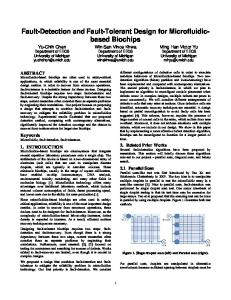
Figure 1: Dilating and shifting of wavelet function.
is adopted. It is necessary to remark that a feature extraction method based on wavelet transform is proposed to do the data preprocessing of the algorithm. The remainder of this paper is organized as follows. In Section 2, we give background knowledge of ITML. Then, wavelet transform is described in Section 3. Section 4 illustrates TE process [20] and gives the experimental results on TE process dataset to demonstrate the good effect of the proposed algorithm. Finally, we draw conclusions and point out future directions in Section 5.
2. Related Work ITML is a metric learning algorithm without eigenvalue computations or semidefinite programming. And the strategy of
Mathematical Problems in Engineering
3
0
Value
0.5
0
400
121
Value
Value
1
120.5
120
500
0 0
500
Sample
500
Value
Value
Value
0.1
0 0
100
0
50
0
500
Sample
0
Sample
(d)
0
500
(f)
60
100
40
50
20
Value
Value
40
0
500
Sample
0
0
Sample
(g)
500 Sample
(e)
60
Value
(c)
0.2
1.5
500 Sample
(b)
2
20
0
Sample
(a)
1
200
500 Sample
(h)
(i)
Figure 2: Observations of fault 12 in the TE process.
regularizing metric in ITML is to minimize the divergence between the target matrix and a given matrix.
The purposeof the ITML is to find a matrix 𝐻 ∈ 𝑅𝐷×𝐷 which satisfies the following pair constraint sets:
Given a dataset {𝑥𝑘 } with 𝑥𝑘 ∈ 𝑅𝐷, 𝑘 = 1, 2, . . . , 𝑛. The Mahalanobis distance between 𝑥𝑖 and 𝑥𝑗 can parameterized by a matrix 𝐻 as follows:
𝐻 ∈ 𝑅𝐷×𝐷, s.t. 𝐷𝐻 (𝑥𝑖 , 𝑥𝑗 ) ≤ 𝑠 (𝑖, 𝑗) ∈ 𝑆,
𝑇
𝐷𝐻 (𝑥𝑖 , 𝑥𝑗 ) = (𝑥𝑖 − 𝑥𝑗 ) 𝐻 (𝑥𝑖 − 𝑥𝑗 ) .
(1)
In ITML, pair constraints are used to represent the relationship of data in the same or different categories. If 𝑥𝑖 and 𝑥𝑗 are in the same categories, the Mahalanobis distance between them should be smaller than a given value 𝑠. Similarly, if 𝑥𝑖 and 𝑥𝑗 are in different categories, the Mahalanobis distance between them should be larger than a given value 𝑏.
(2)
𝐷𝐻 (𝑥𝑖 , 𝑥𝑗 ) ≥ 𝑏 (𝑖, 𝑗) ∈ 𝐷, where 𝑆 and 𝐷 represent the set of pairs of data in the same and different categories, respectively. It deserves pointing out that there will be not only one matrix 𝐻 ∈ 𝑅𝐷×𝐷 which satisfies all the constraints. To ensure the stability of the metric learning, the target matrix 𝐻 is regularized to a given function 𝐻0 . The distance between 𝐻
4
Mathematical Problems in Engineering
0
10 Sample
200
0
20
Value
0.5
0
1000
400
Value
Value
1
0 0
(a)
2
0
10 Sample
0
20
10 Sample
20
20
(f)
50
0
10 Sample
0
200
Value
Value 0
50
(e)
50
0
10 Sample
0
100
100
20
100
0.2
0
20
10 Sample
0
(c)
Value
Value
Value
20
0.4
(d)
Value
10 Sample (b)
4
0
500
0
10 Sample
(g)
20
100
0
0
(h)
10 Sample
20
(i)
Figure 3: Results of the wavelet transform.
and 𝐻0 can be expressed as a type of Bregman matrix divergence [21] as follows: 𝑇
𝐷𝜙 (𝐻, 𝐻0 ) = 𝜙 (𝐻) − 𝜙 (𝐻0 ) − tr ((∇𝜙 (𝐻0 )) (𝐻 − 𝐻0 )) , (3) in which tr(𝐻) denotes the trace of matrix 𝐻 and 𝜙(𝐻) is a given strictly convex differentiable function that plays a determinant role in the properties of the Bregman matrix divergence. Taking the advantages of different differentiable functions into account, 𝜙(𝐻) is chosen as 𝑙𝑜𝑔(det(𝐻)). And the corresponding, Bregman matrix divergence 𝐷𝜙 (𝐻, 𝐻0 ) is called LogDet divergence. According to the further generalization, the LogDet divergence keeps invariant when performing the invertible linear transformation 𝐾, expressed as [22] 𝐷LD (𝐻, 𝐻0 ) = tr (𝐻𝐻0−1 ) − log (det (𝐻𝐻0−1 )) − 𝑛, 𝐷LD (𝐻, 𝐻0 ) = 𝐷LD (𝐾𝑇 𝐻𝐾, 𝐾𝑇 𝐻0 𝐾) .
(4)
The metric learning problem can be translated into a LogDet optimization problem as follows: min 𝐷LD (𝐻, 𝐻0 ) , 𝐻≥0
s.t.
𝑇
tr (𝐻 (𝑥𝑖 − 𝑥𝑗 ) (𝑥𝑖 − 𝑥𝑗 ) ) ≤ 𝑠 (𝑖, 𝑗) ∈ 𝑆,
(5)
𝑇
tr (𝐻 (𝑥𝑖 − 𝑥𝑗 ) (𝑥𝑖 − 𝑥𝑗 ) ) ≥ 𝑏 (𝑖, 𝑗) ∈ 𝐷. It is worth pointing out that distance constraints 𝐷𝐻(𝑥𝑖 , 𝑥𝑗 ) ≤ 𝑠 are equivalent to the linear constraints tr(𝐻(𝑥𝑖 − 𝑥𝑗 )(𝑥𝑖 − 𝑥𝑗 )𝑇 ) ≤ 𝑠. To guarantee the existence of the feasible solution to (5), Kulis proposed an iterative algorithm which introduce slack variable in it [21]. In this way, an iterative equation to update the Mahalanobis distance function is found as follows: 𝑇
𝐻𝑡+1 = 𝐻𝑡 + 𝜇𝐻𝑡 (𝑥𝑖 − 𝑥𝑗 ) (𝑥𝑖 − 𝑥𝑗 ) 𝐻𝑡 ,
(6)
where 𝜇 is a parameter mentioned in Algorithm 1. In the algorithm, the slack variable 𝛽 balanced the satisfaction of min𝐻≥0 𝐷LD (𝐻, 𝐻0 ) and the linear constraints. Learning the
Mathematical Problems in Engineering
5 FI 8
1
A
Condenser
JI
CWS
FI
2
D
XC
TI
XF XG
Analyzer
XH
Stripper Vap/liq separator
TI TI
FI
TI
CWR
12
FI
LI
1 Stm
Reactor Cond
Analyzer
6
XF
4
XD XE XF XG XH
FI
C
XE
FI 10
XE
FI
XD
PI
CWS
XB
XD
XB
PI
CWR
XA
XC
XA
PI
LI
Purge
5
TI
3
E
9
Compressor LI
SC 7
FI
FI
Analyzer
FI
11
Product
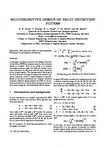
Figure 4: The Tennessee Eastman chemical process. ×10−4 1
1000
SPE
T2
1500
500 0
100
200
300
400
500 600 Sample
700
800
900
(a)
0.5 0
100
200
300
400
500 600 Sample
700
800
900
(b)
Figure 5: The classification accuracy of fault 1 dataset for PCA method.
Mahalanobis matrix 𝐻 based on the given matrix 𝐻0 , we can classify the data using k-nearest neighbor classifier to realize failure diagnosis.
3. Fault Diagnosis Using ITML In the data-driven fault diagnosis system based on the ITML, the system is sensitive to values of the datasets. However, the faults are reflected in vibration amplitude or variation tendency in certain situations. Wavelet transform performs multiscale analysis to the dataset by dilating and shifting the wavelet functions. It transforms the discrepancies of vibration amplitude or variation tendency into the discrepancies of values. Wavelet functions are localized in time and frequency. Wavelet transform has two main advantages. Firstly, the
analysis window changes itself rather than other complex exponential. Secondly, the duration of the analysis window is not fixed. The wavelet functions are created from the wavelet mother function, by dilating and shifting the window. The wavelet mother function 𝜓(𝑡) is a function with zero mean which has limited duration and salutatory duration and amplitude. The wavelet functions can be express as [23] 𝜓𝑎, 𝑏 (𝑡) =
1 𝑡−𝑏 ), 𝜓( √𝑎 𝑎
(7)
where 𝑎 is scaling factor and 𝑏 is translation factor, with 𝑎, 𝑏 ∈ 𝑅, 𝑎 ≥ 0. Through increasing the scaling factor 𝑎, the wavelet function is expanded and is conducive to analysis signals with low frequency and long duration. Correspondingly, by reducing the scaling factor 𝑎, the wavelet function is shrunk and is conducive to analysis signals with high frequency
Mathematical Problems in Engineering 1
1
0.95
0.95 Classification accuracy
Classification accuracy
6
0.9 0.85 0.8 0.75 0.7
0.9 0.85 0.8 0.75
5
10
15
20 25 30 Order of model
35
40
45
0.7
5
(a) FDA method
10 15 kth nearest neighbor
20
25
(b) ITML method
Figure 6: The classification accuracy of fault 1 dataset for 2 methods. (a) The experimental results based on FDA method. (b) The experimental results based on ITML method.
and short duration. By changing the translation factor 𝑏, the wavelet functions can realize the traversal along the time axis to get the information of time domain. The wavelet transform can study different scale features and information of time domain which can be expressed as in Figure 1. The wavelet transform aims at getting a linear combination of the wavelet functions to describe the features in the signal. The value of the wavelet transform is generated by different scaling factors and translation factors. The wavelet transform is defined as [23] WT𝑎, 𝑏 =
1 𝑡−𝑏 ) 𝑑𝑡. ∫ 𝑥 (𝑡) 𝜓∗ ( √𝑎 𝑅 𝑎
(8)
Wavelet transform performs multiscale analysis to the dataset which is conducive to the results of ITML. In order to verify this, a wavelet transform to the dataset of TE process is constructed. TE process is introduced in Section 4. Selecting the corresponding 20 consecutive observations of the 9 variables of fault 12 dataset in the TE process randomly, the results of the wavelet transform are shown in Figures 3 and 4. The red lines in Figures 2 and 3 represent the value of faultfree dataset and the blue lines represent the value of fault 12 dataset. The results of wavelet transform show that features in the signal are converted into the discrepancies of values. Wavelet transform performs well in doing the feature extraction of the ITML.
4. Experimental Results 4.1. Dataset. The designed method of the data-driven fault diagnosis system proposed in this work is applied on the Tennessee Eastman chemical process. TE process is a chemical plant using as an industrial benchmark process; the schematic flow diagram and instrumentation of which are shown in Figure 4 [24]. TE process gets two products from four reactants. All the 52 variables
Table 1: Manipulating variables in TE plant. Variable number XMV (1) XMV (2) XMV (3) XMV (4) XMV (5) XMV (6) XMV (7) XMV (8) XMV (9) XMV (10) XMV (11)
Variable name D feed flow (stream 2) E feed flow (stream 3) A feed flow (stream 1) A and C feed flows (stream 4) Compressor recycle valve Purge valve (stream 9) Separator pot liquid flow (stream 10) Stripper liquid product flow (stream 11) Stripper steam valve Reactor cooling water flow Condenser cooling water flow
contained in the process are 11 control variables and 41 measurement variables, respectively, as listed in Table 1 [16] and Table 2 [16]. 20 process faults and a valve fault are defined in TE process, as shown in Table 3 [16]. In the work of Chiang et al. [15], a widely used dataset of TE process is given. To copy the measurements of 52 variables for 24 hours, 22 training datasets are contained in the dataset corresponding to the fault-free operating condition and 21 fault operating conditions. Simultaneously, 22 test datasets are contained in the dataset, in which the measurements of 52 variables for 48 hours are collected. It is worth pointing out that the faults in the 22 test datasets are added after 8 simulation hours. The sampling time of both of 22 training datasets and 22 test datasets is 3 minutes. 4.2. Performance Comparing with Classical Methods. To demonstrate the advantages of the proposed fault detection method, we compare it to two classical1 methods, PCA and FDA. We carried out experiments on the dataset of TE
Mathematical Problems in Engineering
7
Table 2: Measured variables in TE plant. Variable number XMEAS (1) XMEAS (2) XMEAS (3) XMEAS (4) XMEAS (5) XMEAS (6) XMEAS (7) XMEAS (8) XMEAS (9) XMEAS (10) XMEAS (11) XMEAS (12) XMEAS (13) XMEAS (14) XMEAS (15) XMEAS (16) XMEAS (17) XMEAS (18) XMEAS (19) XMEAS (20) XMEAS (21) XMEAS (22) XMEAS (23) XMEAS (24) XMEAS (25) XMEAS (26) XMEAS (27) XMEAS (28) XMEAS (29) XMEAS (30) XMEAS (31) XMEAS (32) XMEAS (33) XMEAS (34) XMEAS (35) XMEAS (36) XMEAS (37) XMEAS (38) XMEAS (39) XMEAS (40) XMEAS (41)
Variable name A feed (stream 1) D feed (stream 2) E feed (stream 3) A and C feed (stream 4) Recycle flow (stream 8) Reactor feed rate (stream 6) Reactor pressure Reactor level Reactor temperature Purge rate (stream 9) Product separator temperature Product separator level Product separator pressure Product separator underflow (stream 10) Stripper level Stripper pressure Stripper underflow (stream 11) Stripper temperature Stripper steam flow Compressor work Reactor cooling water outlet temperature Separator cooling water outlet temperature Component A (stream 6) Component B (stream 6) Component C (stream 6) Component D (stream 6) Component E (stream 6) Component F (stream 6) Component A (stream 9) Component B (stream 9) Component C (stream 9) Component D (stream 9) Component E (stream 9) Component F (stream 9) Component G (stream 9) Component H (stream 9) Component D (stream 11) Component E (stream 11) Component F (stream 11) Component G (stream 11) Component H (stream 11)
process and the classification accuracy of 𝑘-nearest neighbor is chosen to evaluate the performance of classification. The experiments are conducted on 6 datasets in the TE process, fault-free dataset, fault 1 dataset, fault 2 dataset, fault 4 dataset, fault 6 dataset, and fault 7 dataset, respectively. The feature extraction method of the datasets of TE process is selected as wavelet transform. To balance the performance of the feature extraction with the amount of delay, every 7 consecutive samples are collected to do a wavelet transform.
Table 3: Process faults in TE plant. Fault number IDV (1) IDV (2) IDV (3) IDV (4) IDV (5) IDV (6) IDV (7) IDV (8) IDV (9) IDV (10) IDV (11) IDV (12) IDV (13) IDV (14) IDV (15) IDV (16) IDV (17) IDV (18) IDV (19) IDV (20) IDV (21)
Process variable A/C feed ratio, B composition constant B composition, A/C ration constant D feed temperature Reactor cooling water inlet temperature Condenser cooling water inlet A feed loss C header pressure loss-reduced availability A, B, C feed composition D feed temperature C feed temperature Reactor cooling water inlet temperature Condenser cooling water inlet temperature Reaction kinetics Reactor cooling water valve Condenser cooling water valve Unknown Unknown Unknown Unknown Unknown The valve fixed at steady state position
The slack variable used to avoid the overfitting problem is set as 𝛽 = 10−3 and all results presented are the average over 10 runs. The experimental results of fault 1 dataset are given in Figures 5 and 6. Figure 5 shows the result of fault detection of fault 1 dataset for PCA method when fault occurs in both of the two orthogonal subspaces, which can be successfully detected by 𝑆𝑃𝐸 and 𝑇2 statistics. And the fault detection accuracy of fault 1 dataset for PCA method is 0.99. PCA method provides a satisfactory fault detection rate, but it cannot estimate fault types because it determines the lower dimensional subspaces without considering the information between the classes. Figure 6(a) indicates that the classification accuracy of FDA method float in line with the order of model and the classification accuracy are not totally satisfactory. Figure 6(b) illustrates that the ITML method gives higher fault detection rate than FDA method and it remains stable for different 𝑘th nearest neighbor. Furthermore, ITML method takes advantages of PCA method that it can estimate fault types directly. Experimental results are summarized in Figure 7 and these results reveal that ITML method is more robust than PCA and FDA. Considering the ability of estimating fault types directly, ITML method achieves the best classification accuracy across all datasets. And the performance and effectiveness of the wavelet transform based feature extraction are demonstrated by the results of the experiment.
8
Mathematical Problems in Engineering
Classification accuracy
1
0.95
0.9
0.85
0.8
Fault 1 Fault 2 Fault 4 Fault 6 Fault 7 Fault type PCA FDA ITML
Figure 7: The classification accuracy of 5 different datasets for 3 methods.
5. Conclusion In this paper, we proposed a fault detection scheme based on information-theoretic metric learning. ITML performs well in learning Mahalanobis distance function. In the proposed framework, the feature vector is firstly extracted by applying wavelet transform. After that, we apply the ITML algorithm in fault detection method to improve fault detection accuracy and estimate fault types. Comparing with the fault detection schemes based on PCA and FDA, experiments on TE process dataset demonstrate that the proposed method is more robust. The performance and effectiveness of the wavelet transform-based feature extraction are demonstrated by the results of the experiments at the same time.
Conflict of Interests The authors declared that there is no conflict of interests regarding the publication of this paper.
Acknowledgments The authors acknowledge the support of China Postdoctoral Science Foundation Grant no. 2012M520738 and Heilongjiang Postdoctoral Fund no. LBH-Z12092.
References [1] Z. Xudong, Z. Lixian, S. Peng, and L. Ming, “Stability and stabilization of switched linear systems with mode-dependent average dwell time,” IEEE Transactions on Automatic Control, vol. 57, no. 7, pp. 1809–1815, 2012. [2] Z. Xudong, Z. Lixian, S. Peng, and L. Ming, “Stability of switched positive linear systems with average dwell time switching,” Automatica, vol. 48, no. 6, pp. 1132–1137, 2012.
[3] Z. Xudong and L. Xingwen, “Improved results on stability of continuous-time switched positive linear systems,” Automatica, 2013. [4] S. Yin, S. Ding, A. Haghani, H. Hao, and P. Zhang, “A comparison study of basic datadriven fault diagnosis and process monitoring methods on the benchmark Tennessee Eastman process,” Journal of Process Control, vol. 22, no. 9, pp. 1567–1581, 2012. [5] S. Yin, X. Yang, and H. R. Karimi, “Data-driven adaptive observer for fault diagnosis,” Mathematical Problems in Engineering, vol. 2012, Article ID 832836, 21 pages, 2012. [6] S. Yin, H. Luo, and S. Ding, “Real-time implementation of faulttolerant control systems with performance optimization,” IEEE Transactions on Industrial Electronics, vol. 64, no. 5, pp. 2402– 2411, 2014. [7] R. Dunia, S. J. Qin, T. F. Edgar, and T. J. McAvoy, “Use of principal component analysis for sensor fault identification,” Computers and Chemical Engineering, vol. 20, pp. 713–718, 1996. [8] S. Yin, S. X. Ding, A. H. A. Sari, and H. Hao, “Data-driven monitoring for stochastic systems and its application on batch process,” International Journal of Systems Science, vol. 44, no. 7, pp. 1366–1376, 2013. [9] S. Yin, G. Wang, and H. Karimi, “Data-driven design of robust fault detection system for wind turbines,” Mechatronics, 2013. [10] I. T. Jolliffe, Principal Component Analysis, Springer, Berlin, Germany, 1986. [11] R. O. Duda, P. E. Hart, and D. G. Stork, Pattern Classification, Wiley-Interscience, New York, NY, USA, 2001. [12] D. Zumoffen and M. Basualdo, “From large chemical plant data to fault diagnosis integrated to decentralized fault-tolerant control: pulp mill process application,” Industrial and Engineering Chemistry Research, vol. 47, no. 4, pp. 1201–1220, 2007. [13] J. E. Jackson and G. S. Mudholkar, “Control procedures for residuals associated with principal component analysis,” Technometrics, vol. 21, no. 3, pp. 341–349, 1979. [14] N. D. Tracy, J. C. Young, and R. L. Mason, “Multivariate control charts for individual observations,” Journal of Quality Technology, vol. 24, no. 2, pp. 88–95, 1992. [15] L. H. Chiang, E. L. Russell, and R. D. Braatz, “Fault diagnosis in chemical processes using Fisher discriminant analysis, discriminant partial least squares, and principal component analysis,” Chemometrics and Intelligent Laboratory Systems, vol. 50, no. 2, pp. 243–252, 2000. [16] L. H. Chiang, E. L. Russell, and R. D. Braatz, Fault Detection and Diagnosis in Industrial Systems, Springer, London, UK, 2001. [17] S. Xiang, F. Nie, and C. Zhang, “Learning a mahalanobis distance metric for data clustering and classification,” Pattern Recognition, vol. 41, no. 12, pp. 3600–3612, 2008. [18] L. Meizhu and B. Vemuri, “A robust and efficient doubly regularized metric learning approach,” in Computer Vision—ECCV 2012, pp. 646–659, Springer, Berlin, Germany, 2012. [19] J. V. Davis, B. Kulis, P. Jain, S. Sra, and I. S. Dhillon, “Information-theoretic metric learning,” in Proceedings of the 24th International Conference on Machine learning (ICML ’07), pp. 209– 216, ACM, June 2007. [20] J. J. Downs and E. F. Vogel, “A plant-wide industrial process control problem,” Computers and Chemical Engineering, vol. 17, no. 3, pp. 245–255, 1993. [21] B. Kulis, M. Sustik, and I. Dhillon, “Learning low-rank kernel matrices,” in Proceedings of the 23th International Conference on Machine Learning (ICML ’06), pp. 505–512, ACM, June 2006.
Mathematical Problems in Engineering [22] J. V. Davis and I. Dhillon, “Differential entropic clustering of multivariate gaussians,” Advances in Neural Information Processing Systems, vol. 19, p. 337, 2007. [23] T. A. Ridsdill-Smith, The Application of the Wavelet Transform to the Processing of Aeromagnetic Data, The University of Western Australia, Crawley, Australia, 2000. [24] S. Yin, Data-Driven Design of Fault Diagnosis Systems, VDI, Dusseldorf, Germany, 2012.
9
Advances in
Operations Research Hindawi Publishing Corporation http://www.hindawi.com
Volume 2014
Advances in
Decision Sciences Hindawi Publishing Corporation http://www.hindawi.com
Volume 2014
Journal of
Applied Mathematics
Algebra
Hindawi Publishing Corporation http://www.hindawi.com
Hindawi Publishing Corporation http://www.hindawi.com
Volume 2014
Journal of
Probability and Statistics Volume 2014
The Scientific World Journal Hindawi Publishing Corporation http://www.hindawi.com
Hindawi Publishing Corporation http://www.hindawi.com
Volume 2014
International Journal of
Differential Equations Hindawi Publishing Corporation http://www.hindawi.com
Volume 2014
Volume 2014
Submit your manuscripts at http://www.hindawi.com International Journal of
Advances in
Combinatorics Hindawi Publishing Corporation http://www.hindawi.com
Mathematical Physics Hindawi Publishing Corporation http://www.hindawi.com
Volume 2014
Journal of
Complex Analysis Hindawi Publishing Corporation http://www.hindawi.com
Volume 2014
International Journal of Mathematics and Mathematical Sciences
Mathematical Problems in Engineering
Journal of
Mathematics Hindawi Publishing Corporation http://www.hindawi.com
Volume 2014
Hindawi Publishing Corporation http://www.hindawi.com
Volume 2014
Volume 2014
Hindawi Publishing Corporation http://www.hindawi.com
Volume 2014
Discrete Mathematics
Journal of
Volume 2014
Hindawi Publishing Corporation http://www.hindawi.com
Discrete Dynamics in Nature and Society
Journal of
Function Spaces Hindawi Publishing Corporation http://www.hindawi.com
Abstract and Applied Analysis
Volume 2014
Hindawi Publishing Corporation http://www.hindawi.com
Volume 2014
Hindawi Publishing Corporation http://www.hindawi.com
Volume 2014
International Journal of
Journal of
Stochastic Analysis
Optimization
Hindawi Publishing Corporation http://www.hindawi.com
Hindawi Publishing Corporation http://www.hindawi.com
Volume 2014
Volume 2014