Abstract: In this paper a fault detection (FD) filter design method is proposed for hybrid switched ... technologies have attracted much attention (Chen and Patton.
A Fault Detection Filter Design Method for Hybrid Switched Linear Parameter Varying Systems G. Gagliardi ∗ A. Casavola ∗ D. Famularo ∗ G. Franz`e ∗ ∗ Universit` a
degli Studi della Calabria, Rende (CS), 87036, ITALY (e-mail: {ggagliardi,casavola,famularo,franze}@deis.unical.it)
Abstract: In this paper a fault detection (FD) filter design method is proposed for hybrid switched linear parameter-varying (LPV) systems. The FD filter is designed as a bank of H∞ Luenberger observers, achieved by optimizing frequency conditions which ensure guaranteed level of disturbance rejection and fault sensitivity. The switching signal is assumed to be known and satisfying a dwell-time prescription on the allowable switching sequences which ensures the asymptotical stability of the switched LPV system. The design method is recast as a Semidefinite Programming Problem in the observer bank gains. A FD threshold logic is also proposed in order to reduce the generation of false alarms. A practical example from lateral vehicle dynamics is provided to illustrate the effectiveness of the proposed technique. Keywords: Hybrid Systems, Linear Parameter Varying Systems, Robust Fault Detection, Linear Matrix Inequalities. 1. INTRODUCTION Fault Detection and Isolation techniques are important topics in systems engineering from the viewpoint of improving the system reliability. A fault represents any kind of malfunction in a plant that leads to anomalies in the overall system behavior. Such an event may happen due to process, sensors and/or actuator failures inside the plant. During the last decade, model based fault detection (FD) technologies have attracted much attention (Chen and Patton [1999], Frank et al. [1997], Patton et al. [2000]). Starting from the rich theoretical results and increasing industrial applications it is well known that model-based fault detection can be approached as an output estimation problem and leads to a multiobjective design problem. In order to ensure a quick and reliable detection of faults, both the robustness of the FD systems to model uncertainties, unknown disturbance and its sensitivity to faults must be taken into consideration. In the context of uncertain linear time-invariant (LTI) systems, a number of approaches have been proposed for the design of FD filters (see Frank et al. [1997], Patton et al. [2000], Rambeaux et al. [2000], Casavola et al. [2007] and references therein for a relevant bibliography on the matter). Nonetheless, a huge number of plants exhibit switching phenomena (see Dayawansa and Marlin [1999], Zefran and Burdick [1998]) which can be described by means of a hybrid model paradigm. A hybrid model characterizes a system composed by both continuous and discrete components. The former are typically associated to physical variables and dynamics, the latter with logic devices, such as switches, digital circuitry, software code. Switched systems paradigms have in fact a lot of applications in control of mechanical systems, automotive industry, aircraft and air traffic control, electrical power converters and many other fields. To capture the evolutions of these systems, mathematical models need to combine, in one or another way, both continuous and discrete dynamics in all kinds of variations.
However, they basically consist of a mix of differential or difference equations on one hand and automata, discrete-event models or Petri Nets on the other hand (van der Schaft and Schumacher [2000], Koutsoukos and Antsaklis [2003], Hamdi et al. [2009]). Here, a model-based FD approach for hybrid systems is addressed by exploiting the theory of switching observers, whose literature is rich, e.g. see (Hamdi et al. [2009], Pettersson [2005, 2006], Alessandri and Coletta [2001], Alessandri et al. [2005]). Moving from the previous considerations, the purpose of this paper is to discuss a FD frequency design H ∞ /H − procedure for systems described by a class of linear time-varying models, whose structure jointly commutes according to an external switching signal σ(t) which depends linearly on functions of measurable parameters θ(t) (H-LPV systems), Lim and Chan [2003]. We will suppose that both the measurable parameters and the switching signal are available at each instant time. The FD filter consists here in a bank of time-varying Luenberger observers, doubly tuned with respect to both type of parameters, whose gains are to be found. It will be proved that the H ∞ disturbance decoupling requirement and H − fault sensitivity performance can be easily turned into LMIs in the observer gains and that the H-LPV FD design problem is then solvable by means of standard semidefinite programming procedures. In order to ensure the stability to the overall FD setup, a dwell-time condition on the transition between two consecutive switching events is assumed. The proposed condition extends to the LPV case a previous result proved in a switched LTI framework by Abdo et al. [2010]. As a standard in FD schemes, a decision logic in charge to minimize the rate of false alarms generation is determined via frequency-domain conditions on fictitious doubly-indexed fault/disturbance vs. residual maps (transfer functions), each of them representing a specific transfer function of a LTI system corresponding to a vertex of the polytope family of plants.
Finally, a numerical experiment on a lateral vehicle dynamics with a faulty actuator is finally reported and described in details.
Given such a plant model we want to design a fault detection (FD) system such that:
NOTATIONS
(1) the effects of the process input signal and disturbances are minimized; (2) the effects of the faults are properly enhanced; (3) false alarm occurrences are minimized.
Given a symmetric matrix A = AT ∈ Rn×n we denote respectively with λm (A) and λM (A) the miniminum and maximum eigenvalues. 2. PROBLEM STATEMENT Consider the class of multi-model linear possibly time-varying systems whose system matrices depend linearly on a timevarying parameter vector θ(t) and on a switching signal σ(t). We will suppose also that both parameters may act as scheduling terms. This class of systems is described by x(t) ˙ = Aσ(t) (θ(t)) x(t) + Bσ(t) (θ(t)) u(t) + Eσ(t) (θ(t)) f (t)+ Gσ(t) (θ(t)) d(t)
y(t) = Cσ(t) (θ(t)) x(t) + Dσ(t) (θ(t)) u(t) + Fσ(t) (θ(t)) f (t)+ Hσ(t) (θ(t)) d(t) (1) where • x(t) ∈ Rn denotes the state, u(t) ∈ Rm the control input and y(t) ∈ R p the measured output; • f (t) ∈ Rn f denotes the fault signal, d(t) ∈ Rnd the exogenous disturbance;
On the basis of the previous requirements such a filter must be sensitive with respect to failures, viz. capable to distinguish between faults and unknown disturbances. The design must be accomplished by means of a suitable residual evaluation function which must be close to zero in fault-free conditions and must deviate significantly when a failure occurs. Thanks to the hypotheses that the plant parameter is measurable and the switching signal is directly available, the idea is to build a residual generator as a switched time-varying observer, x(t) ˙ = Aσ(t) (θ(t)) x(t) ˆ + Bσ(t) (θ(t)) u(t)+ L (θ(t)) (y(t) − y(t)) ˆ σ(t) (4) y(t) ˆ = Cσ(t) (θ(t)) x(t) ˆ + Dσ(t) (θ(t)) u(t) r(t) = y(t) − y(t) ˆ which can be characterized as a bank of N time-varying observers by considering all possible realizations of the switching signal. The filter gain Lσ(t) (θ(t)), which is the design parameter of the diagnostic observer, has the following structure
In what follows the following conditions will be assumed: • the fault signal f (t) and the disturbance d(t) are finite energy signals with radius norms belonging to the following proper subsets of L2 , i.e. rZ � � ∞ 2 k f (t)k2 dt ≤ ε f , Ω f , f (·)| ∃ε f > 0 s.t. 0 rZ � � ∞ 2 kd(t)k2 dt ≤ εd Ωd , d(·)| ∃εd > 0 s.t. 0
• the switching signal σ(t) ∈ {1, . . . , N} characterizes the sudden transition of the plant structure and is supposed to be available at each time instant. Assuming N logical states i ∈ {1, . . . , N} existing, σ(t) is piecewise-constant taking one this integer values at each time instant, viz. σ(t) ∈ {1, . . . , N} (2) l • θ(t) ∈ R , is a possibly time-varying parameter which is known to belong to a given simplex Θ , {θ ∈ Rl |
l
∑ θi = 1, 0 ≤ θi ≤ 1,
i = 1, . . . , l}
i=1
and is supposed to be measurable. Notice that, the family of systems (1) consists of a finite set of possibly timevarying models. Then, the system matrices � � Aσ(t) (θ(t)) Bσ(t) (θ(t)) Eσ(t) (θ(t)) Gσ(t) (θ(t)) = Cσ(t) (θ(t)) Dσ(t) (θ(t)) Fσ(t) (θ(t)) Hσ(t) (θ(t)) � j j j j� l A B E G j ∑ θ (t) Cij Dij Fij Hij (3) i i i i j=1 can be defined as a convex combination of the doubleindexed matrices � j j j j� i = 1, . . . , N, Ai Bi Ei Gi j j j j , j = 1, . . . , l Ci Di Fi Hi being known constant matrices.
nθ
Lσ(t) (θ(t)) = Li (θ(t)) =
∑ Lij θ j (t)
(5)
j=1
when the switching signal is equal to σ(t) = i. The gain matrices j Li ∈ R p×n are derived for each couple i, j so that the problem prescriptions are satisfied. When the residual generator (4) is applied to the plant (1), the estimation error e(t) , x(t) − x(t) ˆ and the residual r(t) are governed by the following equation � e(t) ˙ = Aσ(t) (θ(t)) − Lσ(t) (θ(t))Cσ(t) (θ(t)) �e(t) + Eσ(t) (θ(t)) − Lσ(t) (θ(t)) Gξ (θ(t)) �f (t) + Fσ(t) (θ(t)) − Lσ(t) (θ(t)) Hσ(t) (θ(t)) d(t) r(t) = Cσ(t) (θ(t))e(t) + Gσ(t) (θ(t)) f (t) + Hσ(t) (θ(t)) d(t) (6) The filter (4), for each discrete state σ(t) = i, must result asymptotically stable and designed so as to minimize the disturbance effects and enhancement of the fault sensitivity. In order to reduce the occurrence of false alarms, the obtained residuals are then processed by means of an appropriate index Jr , and then evaluated by using a decision logic which acts according to the following rules Jr < Jth , for f (t) = 0
(7)
Jr ≥ Jth , for f (t) 6= 0 (8) Fault-detection decisions are based on the evaluation of the characteristics of the residual signals. To this end, the following frequency domain evaluation function is introduced �1 � Z ωs 2 1 ∗ (9) r ( j ω) r( j ω) d ω Jr , 2 π (ωs − ωi ) ωi
The frequency window [ωi , ωs ] is a-priori selected by the designer, even if a suitable choice could increase the robustness and the fault detection capabilities of the residual observer.
3. HYBRID LPV STABILITY CONDITIONS In what follows, a dwell-time condition which ensures the stability of the overall switched system, provided that the individual LPV subsystems are quadratically stable, is presented. The result here outlined is a direct extension to the LPV case of similar conditions derived in Abdo et al. [2010] for switching LTI plants. The idea is that asymptotical stability can be proved if the switching rate is sufficiently slow and the transient effects occurring after each switch are dissipated. To this end, the following definitions of dwell-time and average dwell-time are of interest (see Liberzon et al. [1999], Hespanha et al. [1999], Morse [1996] for a detailed analysis on the matter). Definition 1. Dwell-Time. Let t1 ,t2 , . . . ,tN be the switching time instants for the switching signal σ(t). Then, the switching system has a dwell-time τd > 0 if it satisfies ti+1 − ti ≥ τd for all i. A lower-bound on τd can be explicitly calculated from the exponential decay bounds derived from quadratic stability checks on the LPV matrices of the individual subsystems corresponding to each i-th logical state. The stability of slow-switching LPV systems can be ensured if the interval between any two consecutive switching is no smaller than τd . This result comes from the following Lemma which is a simple extension to the LPV case of a Lemma proved by Morse [1996], Abdo et al. [2010] for the switching LTI framework: Lemma 1. Let {A p (θ) : p ∈ P, θ ∈ Θ} be a closed, bounded set of real, n ×�n matrices such that, for a given value of p and θ, A p (θ) ∈ co A1p , . . . , Alp . Suppose that for each p ∈ P, the LPV system x(t) ˙ = A p (θ(t)) x(t) is quadratically stable and let a p and λ p be any finite, nonnegative and positive numbers, respectively, for which j max eA p t ≤ ea p −λ p t , t ≥ 0 (10)
(t, T ). Assume there exist two positive numbers No and τa such that T −t Nσ (T,t) ≤ No + , ∀T ≥ t ≥ 0 (15) τa where No is the chatter bound. Then, τa is the average dwelltime of σ(t). Note that the respect of either the dwell-time or the average dwell-time conditions implies in practice to keep active each observer of the bank for at least τd or τa time instants in the FD filter before a switch to a different observer of the bank could take place. 3.1 Multiple Lyapunov Functions Stability The use of multiple Lyapunov functions is a useful tool for proving stability of a switched systems, (Hespanha [2004], Zhai et al. [2000, 2004]). Consider the hybrid switched linear system x(t) ˙ = Aσ(t) (θ(t)) x(t) (16) We assume that all LPV subsystems of (16) are quadratically stable. Note that the stability of all subsystems is not sufficient to ensure the stability for the whole system. j
If we can find a positive λi such that Ai + λi I, j = 1, . . . , l 1 , is still Hurwitz stable (Aσ (θ) = Ai (θ), when σ = i) then there are symmetric positive definite matrices P1 , . . . , PN such that j
(1) V˙i ≤ −2λiVi (2) there exists constant scalars α2 ≥ α1 > 0 such that
j=1,...,l
Suppose that τd is a number satisfying � � ap τd > sup p∈P λp
|Φ(t, µ)| ≤ e(a−λ(t−µ)) , ∀t ≥ µ ≥ 0
α1 kxk2 ≤ Vi (t) ≤ α2 kxk2 , ∀x ∈ Rn , ∀i ∈ {1, . . . , N} (3) there exists a constant scalar µ ≥ 1 such that Vi (t) ≤ µV j (t), ∀x ∈ Rn , ∀i, j ∈ {1, . . . , N}
(11)
For any admissible switching signal σ(t) : [0, ∞) → P with dwell-time no smaller than τd , the state transition matrix of Aσ(t) satisfies
The first property is a straightforward consequence of (18), while the second and the third hold for α1 =
(12)
where sup p∈P {a p } � � ap λ = in f p∈P λ p − τd
(13)
λ ∈ (0, λ p ], p ∈ P
(14)
j
(Ai + λi I)T Pi + Pi (Ai + λi I) < 0, j = 1, . . . , l (17) By using the solution Pi of (17), one can ensure the stability of the switched system (16) by introducing a Multiple Lyapunov Functions (MLF) candidate Vσ (t) = x(t)T Pσ(t) x(t) (18) and exploiting the following properties (for a proof see e.g. Morse [1996]):
inf
i∈{1,...,N}
λm (Pi ) α2 =
a =
Moreover
(19)
α2 α1
(20)
lnµ 2(λ∗ −λ) ,
whit λ ∈
µ= The dwell-time can be computed as τd = (0, mini (λi )) and λ∗ ∈ (λ, mini (λi )).
Thus, if the switching signal σ(t) “dwells” at each of its value σ(t) = 1, 2, ..., N long enough for the norm of the state transition matrix A p , to drop to at least τd time units, then the hybrid system . . . x(t) = Aσ(t) (θ(t)) x(t) is exponentially stable having a decay rate λ which is upper bounded by the smallest of the decay rates of the LPV system collection x(t) ˙ = A p (θ(t)) x(t), p∈P Definition 2. Average Dwell-time. Let Nσ (T,t) be the number of discontinuities of the switching signal σ(t) on the interval
λM (Pi )
sup i∈{1,...,N}
4. RESIDUAL GENERATOR DESIGN The design of the residual observer (5) is accomplished by solving a multi-objective optimization problem. Starting from the discussion of the above Section, it is possible to restate the fault detection design problem as follows:
H-LPV-FD Note that it is always possible to choose λi because this quantity is upper j T, j bounded by max j=1,...,l 21 λm (Ai + Ai ) .
1
Given a Lyapunov function Vσ (t) = xT (t) Pσ(t) x(t), j Li
(21)
Rn×p ,
find observer matrix gains ∈ i = 1, . . . , N, j = 1, . . . , l and two positive scalars α and β solutions of the following LMI optimization problem j
min a1 α2 − a2 β2
(22)
Li ∈Rn×p
joint availability of the switching signal σ(t) and the plant parameter θ(t). Notice also that the existence, at each time instant t, of a family of observer gains for each mode i l
Li (θ) =
∑ θ j (t) Lij
j=1
solutions of H-LPV-FD, implies the observability of each j j doubly indexed couples (Aˆ i , Li ) (disturbance rejection) and j j (A˜ i , Li ), (fault sensitivity) i = 1, . . . , N, j = 1, . . . , l. 2
s.t.
5. THRESHOLD COMPUTATION � Z ∞� dVσ (t) −
0
dt
0
dt
� Z ∞� dVσ (t)
dt
Z ∞ 0
α2 kd(t)k22 − krd (t)k22 dt
(23)
2 β2 k f (t)k22 − r f (t) 2 dt
(24)
where a1 , a2 are proper positive weights, rd (t) the fault-free residual evolution associated to � e˙d (t) = Aˆ σ (θ) − Lσ (θ) Cˆσ (θ)� ed (t)+ Eˆσ (θ) − Lσ (θ) Fˆσ (θ) d(t) rd (t) = Cˆσ (θ) ed (t) + Fˆσ (θ) d(t) whereas r f (t) the disturbance-free residual associated to � e˙ f (t) = A˜ σ (θ) − Lσ (θ) C˜σ (θ) �e f (t)+ G˜ σ (θ) − Lσ (θ) H˜ σ (θ) f (t) rd (t) = C˜σ (θ) e f (t) + H˜ σ (θ) f (t)
(25)
(26)
The hatted (ˆ·) and tilded (˜·) variables denote a representation where the respective residuals rd (t) and r f (t) have been processed by proper window filters Qd (s) and Q f (s) characterizing the disturbance and fault effects in specific frequency ranges of interest. Inequalities (23) and (24) characterize the usual tradeoff between disturbance decoupling and minimum fault sensitivity achievements usually addressed in the H ∞ /H − approach. The H-LPV-FD design problem can be turned into a Linear Matrix Inequality optimization procedure and the following Proposition reports explicitly the LMI conditions under which problem H-LPV-FD can be checked for admitting a solution: Proposition 1. The inequalities (23) and (24) are satisfied if there exit a family of matrices Pi = PiT , i = 1, . . . , N and maj trix gains Ki ∈ Rn×p , i = 1, . . . , N, j = 1, . . . , l such that the following 2 l N linear matrix inequalities � � T, j j j j j He Pi Aˆ i − Ki Cˆi + Cˆi Cˆi Pi Gˆ i − Kij Hˆ ij + CˆiT, j Hˆ ij �0 ∗
T, j j Hˆ i Hˆ i − α2 I
(27) � T, j ˜ j j j ˜j j j T, j j i ˜ ˜ ˜ He Pi Ai − Ki Ci + Ci Ci Pi E˜ − Ki F˜i + Ci F˜i �0 T, j j ∗ −F˜i F˜i − β2 I (28) (He (X) := X + X T ), i = 1, . . . , N, j = 1, . . . , l, hold true with j j Li = Pi−1 Ki , i = 1, . . . , N, j = 1, . . . , l.
�
Remark 1 - It is worth pointing out that the set of linear matrix inequalities (27) and (28) has been obtained by assuming the
The threshold decision logic is based on the evaluation of the quantity Jth (eqs. (7) and (8)) in order to minimize the occurrence of false alarms. Such a term is derived in fault free conditions according to the time function residual evaluation s Z ωs 1 Jr (t) , r∗ ( j ω) rt ( j ω) dω (29) 2 π (ωs − ωi ) ωi t where rt ( j ω) denotes the Fourier Transform of the residual signal up to time t. From a computational point of view, Jr (t) can be easily obtained by means of standard highly efficient Fast Fourier Transform (FFT) algorithms, available with c MATLAB . Given Jr (t), the threshold can be computed by defining the following doubly indexed family of LTI systems � � ��−1 � � j j j j j j j j Gi j (s) , Cˆi s I − Aˆ i − Li Cˆi Gˆ i − Li Hˆ i + Hˆ i , i = 1, . . . , N, j = 1, . . . , l.
(30)
Due to the fact that the disturbance d(t) is a finite energy signal we also have s
1 (31) sup max Gi j (s) ∞ kdk2 Jth , 2 π (ωs − ωi ) d∈Ωd i=1,...,N j=1,...,l
Then, a computable upper-bound to Jth can be easily achieved by observing that
(1) the scalar α, which is part of the solution of the LMI procedure obtained from problem H-LPV-FD is an upper bound to
Gi j (s) ≤ α, ∀i, j (32) ∞ (2) the set Ωd is upper-bounded, in term of energy norm, by εd The consequence is that Jth ≤
s
1 α εd 2 π (ωs − ωi )
(33)
in healthy situations. Note finally that, the process input u(t) does not appear in the residual generation function and it is, as a consequence, a decoupled input. It is then reasonable to consider a fixed threshold Jth instead of computing a more involved (and not necessary here w.r.t. u(t)) adaptive residual evaluation function. 6. SIMULATION RESULTS Simulation studies on a vehicle lateral dynamical system (see Figure 1) are carried out to illustrate the effectiveness of the proposed method to design an H-LPV filters for robust fault detection purposes via LMIs.
The model used here is the so-called one-track model, aka bicycle model. One-track models are derived upon the assumption that the vehicle is simplified as a point mass with the center of gravity on the ground, which can only move along the x, y axes, and yaw around the z axis. By considering the vehicle side slip
The dwell-time value, computed as in section (3.1), is τd = 1.4774. 35
σ(Gyd(jω)) σ(Gyf(jω))
30 Singular Values (dB)
25 20 15 10 5 0 0 10
If the velocity v varies, the LTI model (34) is replaced with an LPV model in which the longitudinal velocity is a time varying parameter, (Rajamani [2006]). Furthermore, if we consider the velocity range R = [10, 90] and we split the interval in three sub-ranges R1 = [10, 30), R2 = [30, 60) and R3 = [60, 90], the model (34) can be viewed as a three mode (σ = 1, 2, 3) hybrid switching linear parameter varying system. For each σ we assume that the longitudinal velocity is limited by the following constraints + v− (35) σ ≤ vσ ≤ vσ σ = 1, 2, 3 Moreover, we consider three categories of fault on the steering angle measurement δL , each one for a specific system mode σ = 1, 2, 3: fσ=1 (t) = { 0, t ≤ 5s; 1, t > 5s; fσ=2 (t) = { 0, t ≤ 25s; 1, t > 25s; fσ=3 (t) = { 0, t ≤ 50s; 1, t > 50s; The frequency window, where the residual signals r(s) are evaluated, has been chosen equal to [ωi , ωs ] = [0, 25] rad/s. This choice corresponds to the following filters ωs s2 + s + ωs Qd (s) = 2 , Q (s) = f s + 1.4ωs s + ω2s s2 + ωs s + ωs
3
4
10
10
Fig. 2. Singular values plots of Gyd ( jω) and Gyd ( jω)
60 40
Singular Values (dB)
20 0 −20 −40 −60 −80 −100
Q1(jω)σ(Gyd(jω)) Q (jω)σ(G (jω)) 2
yf
−120 −1 10
0
1
10
2
3
10 10 Frequency (rad/sec)
4
10
10
Fig. 3. Singular values plots of Q1 ( jω)Gyd ( jω) and Q2 ( jω)Gyd ( jω) The evolutions of system modes and relevant variables are reported in Figure 4. In this figure we can observe the effectiveness of the proposed solution.
3 σ(t)
angle β and the yaw rate r to be the state variables, the lateral acceleration ay and yaw rate r the output variables, the steering angle δL the input variable, the state space representation of the one track model is given by # " β(t) x(t) ˙ = Ax(t) + Bu(t) + E f (t) + Gd(t), x(t) = r(t) (34) # " ar (t) , u(t) = δL (t) y(t) = Cx(t) + Du(t), y(t) = r(t) where C Cαv +CαH lH CαH − lV Cαv αv − − 1 mv mv2 mv A= lH CαH − lV Cαv lV2 CαV + lH2 CαH B = lV Cαv Iz Iz Iz v Cαv Cαv +CαH lH CαH − lV Cαv − D= m G=B C= m mv 0 0 1
2
10 Frequency (rad/sec)
2
1 0
10
20
30
40
50
60
70
30 40 Time[sec] (b)
50
60
70
(a) 6
4 r(t)
Fig. 1. Kinematics of one-track model
1
10
2
0 0
10
20
Fig. 4. Evolution of mode (a) and detection signal (b) The threshold Jth (dashed line) and the Jr (t) response (continuous line) are depicted in Figure 5. The filter seems to exhibit very good disturbance decoupling properties.
r
J (t)
σ(t)
Koutsoukos X.D. and Antsaklis P.J. “Hybrid Dynamical Systems: Review and Recent Progress”. Software-Enabled Con3 trol: Information Technologies for Dynamical Systems, Wiley-IEEE Press, 2003. 2 Hamdi F., Manamanni N., Messai N., Benmahammed K. “Hy1 brid observer design for linear switched system via Differen0 10 20 30 40 50 60 70 tial Petri Nets”. Nonlinear Analysis: Hybrid Systemsm Vol. (a) 3, pp. 310-322, 2009. 0.4 Lim S. and Chan K. “Analysis of Hybrid Linear Parameter0.3 Varying Systems”. Proceedings of the American Control J th 0.2 Conference, Denver, CO, USA, pp.4822-4827, 2003. Liberzon D. and Morse A. S. “Basic Problems in Stability 0.1 and Design of Switched Systems”. IEEE Control Systems 0 0 10 20 30 40 50 60 70 Time[sec] Magazine, Vol. 19, No. 5, pp. 59-70, 1999. (b) Decarlo R.A., Branicky M.S., Petterson S. and Lennartson B. “Perspectives and Results on the Stability and Stabilizability Fig. 5. Evolution of mode (a), threshold Jth (dashed line) and of Hybrid Systems”. Proceeding of the IEEE, Vol. 88, No. 7, frequency-windowed norm Jr (t) (continuous line) (b) pp. 1069-1082, 2000. Hespanha J.P.. “Uniform Stability of Switched Linear Systems: 7. CONCLUSION Extensions of LaSalles Invariance Principle”. IEEE Transactions on Automatic Control. Vol. 49. pp, 470-482, 2004. A novel Robust FD strategy for hybrid switched linear parametervarying systems has been proposed. By taking advantage of Liberzon D. “Stabilizing a linear system with finite-state hybrid output feedback”. Proceedings of the 7th Mediterranean the Multiple Lyapunov Functions stability concept and using Conference on Control and Automation (MED99), 1999. congruence transformations, the FD design problem has been converted into a tractable LMI optimization problem. A fixed Pettersson S. “Switched State Jump Observer For Switched Systems”. Proceedings of the 16th IFAC World Congress, threshold logic has been proposed in order to to discriminate Prague, 2005. between real and false alarms. A numerical example showing the effectiveness of the proposed approach have been described Pettersson, S. “Designing Switched Observers For Switched System Using Multiple Lyapunov Functions and Dwellin details where the results have shown good detection capabilTime”. Preprints of the 2nd IFAC Conf. on Analysis and ities of the FD logic. Design of Hybrid Systems (Alghero, Italy), 7-9 June 2006. Alessandri A. and Coletta P. “Switching observers For REFERENCES Continuous-Time and Discrete-Time Linear Systems”. ProAbdo A., Damlakhi W., Saijai J. and Ding S., “Design of ceedings of the American Control Conference, Arlington Robust Fault Detection Filter for Hybrid Switched Systems”, VA, USA, June 25-27, pp. 2516-2521, 2001. Proc. of the 2010 Conference on Control and Fault Tolerant Alessandri A., Baglietto M., and Battistelli G. “Luenberger Systems, Nice, France, 2010. Observers for Switching Discrete-Time Linear Systems”. Chen J. and Patton R.J. “Robust Model-Based Fault DiagnoProceedings of the joint 44th IEEE Conference on Decision sis for Dynamic Systems”. Kluwer Academic Publishers: and Control - European Control Conference 2005, Seville, Boston, MA, USA, 1999. Spain, pp. 7014-7019, 2005. Frank, P. M and Ding, X. Survey of robust residual generation Hespanha J. P. and Morse A. S. “Stability of Switched Systems and evaluation methods in observer-based fault detection with Average Dwell-Time”. Proceedings of the 38th IEEE systems. survey and some new results. Journal of Process Conference on Decision and Control, Phoenix AR, USA, pp. Control 7(6),403–424, 1997. 2655-2660, 1999. Patton, R.J., Frank, P.M. and Clark, R.N. (Eds.) Issues of Fault Morse A. S. “Supervisory Control of Families of Linear Set Diagnosis for Dynamic Systems, Springer, 2000. Point Controllers - Part 1: Exact Matching”. IEEE TransacRambeaux, F., Hamelin, F. and Sauter, D. Optimal thresholding tions on Automatic Control, Vol. 41, No. 10, pp. 1413-1431, for robust fault detection of uncertain systems. International 1996. Journal of Robust and Nonlinear Control 10, 1155–1173, Zhai G., Hu B., Yasuda K. and Michel A. N. “Piecewise 2000. Lyapunov Functions for switched Systems with Average Casavola A., Famularo D., Franz`e G. and Sorbara M. “A faultDwell-Time”. Asian Journal of Control, Vol. 2, No. 3, pp. detection, filter-design method for linear parameter-varying 192-197, 2000. systems”, Proc. IMechE - Journal of Systems and Control Zhai G., Lin H., Michel A. N. and Yasuda K. “Stability Engineering, 221, pp. 865-873, 2007. Analysis for Switched Systems with Continuous-Time and Dayawansa W.P. and Marlin C.F., “A converse Lyapunov theoDiscrete-Time Subsystems”. Proceeding of the 2004 Amerirem for a class of dynamical systems which undergo switchcan Control Conference, Boston MA, USA, pp. 4555-4560, ing” . IEEE Trans. Automat. Contr. vol. 44, pp. 751-760, 2004 1999. Rajamani R. “Vehicle Dynamics and Control”, Springer Verlag, Zefran M. and Burdick J.W., “Design of switching controllers 2006. for systems with changing dynamics”, Proc. of the 37th IEEE Conference on Decision and Control, pp. 2113-2118, 1998. van der Schaft A. and Schumacher H. “An Introduction to Hybrid Dynamical Systems”. Lecture Notes in Control and Information Sciences, vol. 251, Springer-Verlag, 2000.