Microstructural Randomness Versus Representative Volume Element in Thermomechanics M. Ostoja-Starzewski Department of Mechanical Engineering, McGill University, 817 Sherbrooke Street West, Montre´al, Que´bec H3A 2K6, Canada e-mail:
[email protected] Fellow ASME
1
Continuum thermomechanics hinges on the concept of a representative volume element (RVE), which is well defined in two situations only: (i) unit cell in a periodic microstructure, and (ii) statistically representative volume containing a very large (mathematically infinite) set of microscale elements (e.g., grains). Response of finite domains of material, however, displays statistical scatter and is dependent on the scale and boundary conditions. In order to accomplish stochastic homogenization of material response, scaledependent hierarchies of bounds are extended to dissipative/irreversible phenomena within the framework of thermomechanics with internal variables. In particular, the freeenergy function and the dissipation function become stochastic functionals whose scatter tends to decrease to zero as the material volume is increased. These functionals are linked to their duals via Legendre transforms either in the spaces of ensemble average velocities or ensemble-average dissipative forces. In the limit of infinite volumes (RVE limit (ii) above) all the functionals become deterministic, and classical Legendre transforms of deterministic thermomechanics hold. As an application, stochastic continuum damage mechanics of elastic-brittle solids is developed. 关DOI: 10.1115/1.1410366兴
Introduction
Presence of dissipative phenomena in mechanics of solids and fluids necessitates a formulation of continuum mechanics consistent with principles of thermodynamics; such a theory is briefly called thermomechanics or continuum thermodynamics. As lucidly and comprehensively elaborated in a recent book by Maugin 关1兴, this challenge conventionally leads to a consideration of one of four continuum thermodynamics: • • • •
thermodynamics of irreversible processes 共TIP兲; thermodynamics with internal variables 共TIV兲; rational thermodynamics 共RT兲; and extended 共rational兲 thermodynamics 共ET兲.
A feature common to all of these approaches is a postulate of existence of a representative volume element 共RVE兲. In other words, we are looking here at deterministic, homogeneous continuum theories, without clear account of random microstructures which are, in fact, prevalent in real materials. While we recognize here that some statistical treatments were carried out as a bridge from micro to macro levels for select variants of the above theories 共e.g., 关2,3兴兲, such studies were concerned with providing foundations from the standpoint of statistical physics directly to the level of the RVE, without making clear what the size of the RVE actually was. On the other hand, homogenization procedure invoked to pass to the RVE in studies of plasticity and damage 共e.g., 关4,5兴兲 always involves a periodic microstructure; see also 共关6兴兲 for other physical problems, and 共关7兴兲 for elastic/ inelastic problems in composites. Some finite scale periodicity in random microstructures is also invoked in theoretical and numerical studies of the RVE size 共关8,9兴兲; in fact, this assumption allows homogenization of elastic materials on very small length scales. Contributed by the Applied Mechanics Division of THE AMERICAN SOCIETY OF MECHANICAL ENGINEERS for publication in the ASME JOURNAL OF APPLIED MECHANICS. Manuscript received by the ASME Applied Mechanics Division, Aug. 31, 2000; final revision, June 12, 2001. Associate Editor: J. W. Ju. Discussion on the paper should be addressed to the Editor, Professor Lewis T. Wheeler, Department of Mechanical Engineering, University of Houston, Houston, TX 77204-4792, and will be accepted until four months after final publication of the paper itself in the ASME JOURNAL OF APPLIED MECHANICS.
Journal of Applied Mechanics
While in plasticity the approach to RVE in a random microstructure may be rapid 共关10兴兲, this is not so for damage phenomena where presence of scatter is evident for even the largest specimens that can be handled in the laboratory, e.g., 共关11,12兴兲. In fact, the dichotomy between statistical damage models motivated by such observations and continuum damage mechanics based on the deterministic TIV formalism is perceived as one of the grand challenges of damage mechanics 共关13,14兴兲. This is one of major motivations of this paper. As theoretical models we first consider strict-sense and widesense stationary random fields, possessing ergodic properties. Many models of microstructural randomness—e.g., Boolean models and tessellations—possess such homogeneity and ergodic characteristics, and they are highly desirable in stochastic homogenization. Real materials, however, often lack these nice behaviors, and, as illustrated by measurements on machine made paper, one may have to work with quasi-stationary and quasi-ergodic random fields. As a guidance in setting up a statistical volume element 共SVE兲 and its deterministic limit, the RVE, in thermomechanics we take the work on elastic microstructures carried out over the last decade, that relies on the Hill condition 共关15兴兲. In essence, it says that the RVE response is independent of the type of boundary conditions applied to it 共i.e., uniform stress or uniform strain or their orthogonal combination兲. For finite-size—which we call mesoscale—material domains the Hill condition leads to three types of boundary conditions 共关16兴兲, and three types of apparent responses: uniform kinematic, uniform traction, and uniform mixed 共orthogonal兲. It follows that in the case of dissipative behaviors, we must primarily consider boundary conditions of uniform dissipative force or uniform velocity. As continuum thermodynamics setting we take TIV, and, in particular, its variant due to Ziegler 关17兴 共also 关18兴兲 which defines a broad class of continuous media from the free energy and dissipation functions 共关19兴兲. In many cases, the uniform kinematic and uniform traction boundary conditions, respectively, bound the effective 共in the macroscopic/global sense兲 dissipative response from above and below; the larger are the mesoscale domains of the material considered, the tighter are the bounds. These bounds, define a sequence of SVE, convergent to the RVE, and serving as a basis of statistical continuum models. We discuss the bounds for
Copyright © 2002 by ASME
JANUARY 2002, Vol. 69 Õ 25
thermal conductivity and damage phenomena. While mathematically at any finite mesoscale the bounds are distinct, the approach to RVE, with increasing window size, to the effective 共macroscopic兲 response, depending on the dissipative process considered, may be very rapid, moderate, or very slow. Furthermore, the free energy may display a different scaling trend than the dissipation function for a given microstructure.
2 Representative Volume Element „RVE… Postulate and Structure of Random Media 2.1 Homogeneous and Ergodic Random Media. Let us first recall the classical assumption of a representative volume element 共RVE兲 according to Hill 关15兴: it is ‘‘a sample that 共a兲 is structurally entirely typical of the whole mixture on average, and 共b兲 contains a sufficient number of inclusions for the apparent overall moduli to be effectively independent of the surface values of traction and displacement, so long as these values are ‘macroscopically uniform.’ ’’ In other words, we need, respectively: 共a兲 statistical homogeneity and ergodicity of the material; these two properties assure the RVE to be statistically representative of the macroresponse 共e.g., 关20,21兴兲; 共b兲 some scale L of the material domain, sufficiently large relative to the microscale d 共inclusion size兲 so as to ensure the independence of boundary conditions. Mechanics of random media, together with probability theory, provides a rigorous setting for study of these issues 共e.g., 关22兴兲. That is, the field problem of random medium B⫽ 兵 B 共 兲 ; 苸⍀ 其
(2.1)
is governed by an equation L共 兲 u⫽f
苸⍀
(2.2)
accompanied by appropriate boundary and/or initial conditions. Here L共兲 is a random field operator 共with randomness caused by, say, elastic moduli being a random field兲, u is a solution field, and f is forcing function. Parametrization by 共element of the sample space ⍀, endowed with a probability measure P兲 indicates the source of uncertainty. Clearly, there are two more basic ways to introduce randomness in a mechanics problem: • randomness in the forcing function—replacing 共2.2兲 by Lu ⫽f( )—as exemplified by problems of random vibrations; • randomness of boundary and/or initial conditions. As we are interested here in the case described by 共2.2兲, we note that each of the realizations B( ) follows laws of deterministic mechanics in that it is a specific heterogeneous material sample. The problem of setting up the RVE of volume V⫽L D 共D is space dimension兲, in the sense of 共a兲 and 共b兲 above, in a global boundary value problem on length scales L macro is illustrated with the help of Fig. 1; of course only one B( ) is shown. In essence, we want
具 L⫺1 典 ⫺1 u⫽f
(2.3)
with independence of boundary conditions as posited by Hill’s condition, on length scale L satisfying dⰆLⰆL macro .
(2.4)
If that is the case, one can then simply deal with a deterministic continuum thermomechanics problem on scale L macro . Hereinafter we assume the microstructure to be characterized by a single correlation radius l c , such as the mean separation between the fibers in a fiber-matrix composite, or mean grain size d. Both inequalities in 共2.4兲 jointly ensure separation of scales in the deterministic continuum mechanics model. The first inequality may be relaxed to d⬍L because we may be considering a micro26 Õ Vol. 69, JANUARY 2002
Fig. 1 Passage from a discrete system of tungsten-carbide „black… and cobalt „white… „a… to an intermediate continuum level „b… involving a mesoscale finite element, that serves as input into the macroscale model accounting for spatial nonuniformity. Figures „a… and „b… are generated by a Boolean model of Poisson polygons and a diffusion random function, respectively „†45‡….
structure with periodic 共or nearly periodic兲 geometry, though possessing some randomness on the level of the unit cell: see relations 共2.8兲–共2.9兲 below. Evidently, the material property 共or properties兲 ⌰ of B( ) entering the continuum mechanics model are to be described by a random field over the D-dimensional space (D⫽1, . . . ,3) ⌰:RD ⫻⍀→R1 .
(2.5)
There exist two types of statistical homogeneity: strict-sense stationarity 共SSS兲 and wide-sense stationarity 共WSS兲. In the first case we are assured of the invariance of any finite-dimensional probability distribution of ⌰ with respect to arbitrary shifts F x1 , . . . ,xm 共 1 , . . . , m 兲 ⫽F x1 ⫹x⬘ , . . . ,xm ⫹x⬘ 共 1 , . . . , m 兲 ᭙x⬘ 苸RD .
(2.6)
This is a very restrictive property. On the other hand, in the WSS case, we have invariance of the mean only with respect to such shifts, along with the dependence of two-point correlation functions on the interpoint separations only, that is 共具 典 denotes ensemble average兲, • mean 具 ⌰(x) 典 ⫽const; • for any two points x1 ,x2 苸RD , the correlation function K ⌰ (x1 ,x2 )⬅ 具 关 ⌰(x1 )⫺ 具 ⌰(x1 ) 典 兴关 ⌰(x2 )⫺ 具 ⌰(x2 ) 典 兴 典 satisfies K ⌰ 共 x1 ,x2 兲 ⫽K ⌰ 共 x1 ⫺x2 兲 .
(2.7)
Clearly, a much wider class of microstructures is described by WSS random fields then SSS random fields, and, as we shall see in the next sections, the former are sufficient for the RVE. Following Eq. 共2.4兲, we mentioned the microstructure with periodic geometry, possessing some randomness on the level of the unit cell. An appropriate model is then offered by a strict-sense 共SS兲 cyclostationary random field, which, for a planar system of square L⫻L unit cells, is stated as Transactions of the ASME
F x1 ⫹mL, . . . ,xm ⫹mL共 1 , . . . , m 兲 ⫽F x1 , . . . ,xm 共 1 , . . . , m 兲
(2.8)
where L is a shift vector 共in any combination of directions along the coordinate axes兲, and m is any integer. Andy Warhol’s 1972 creation S&P Green Stamps is helpful in visualizing this. When the microstructure has an imperfectly periodic geometry, in addition to possessing some randomness on the level of the unit cell, then one should use a wide-sense 共WS兲 cyclostationary random field, which for a system of square unit cells is stated as
具 ⌰ 共 x⫹mL兲 典 ⫽ 具 ⌰ 共 x兲 典
(2.9)
K 共 x1 ⫹mL,x2 ⫹mL兲 ⫽K 共 x1 ,x2 兲 where L is the same as in 共2.8兲, and m is any integer. Returning to the WSS fields, we note that, to ensure the equivalence of macroscopic responses between all the realizations of the ensemble B, an ergodic random field is required. That is, we want any realization to be sufficient to get the ensemble average from the spatial average 共denoted by ⫺ 兲
具 ⌰ 共 x兲 典 ⫽
冕
⍀
⌰ 共 兲 d P 共 兲 ⫽ lim V→⬁
1 V
冕
⌰ 共 ,x兲 dV⫽⌰ 共 兲 .
V
(2.10) In practice 共2.10兲 holds only with some accuracy, and the limiting process V→⬁ cannot truly be carried out. The latter can be discontinued in the regions whose dimension L⫽V 1/D is large compared with the correlation radius l c , so that 共2.4兲 is rewritten as l c ⰆV 1/D ⬃LⰆL macro .
(2.11)
We assume K ⌰ to satisfy 共with probability one兲 ergodic properties with respect to the mean and the correlation function, that is 1 lim V V→⬁ lim V→⬁
1 V
冕
V
冕
V
⌰ 共 x, 兲 dV⫽m⫽ 具 ⌰ 共 x, 兲 典 (2.12)
In practice, the left and right-hand sides of 共2.12兲1 and 共2.12兲2 would be replaced, respectively, by a spatial average from a finite number of sampling points taken over one realization N
兺
(2.13)
and an ensemble average from a finite number of realizations taken at one sampling point N
1 ⌰ 共 x, n 兲 . 具 ⌰ 共 x兲 典 ⫽ N n⫽1
兺
(2.14)
The ergodicity of these estimators—i.e., ⌰(x, )⫽ 具 ⌰(x, ) 典 —is assured, for sufficiently large N, by the property of the correlation function lim K ⌰ 共 ⌬x兲 ⫽0.
(2.15)
兩 ⌬x兩 →⬁
This, for instance, is the case with Voronoi mosaics based on a Poisson point field, both in two dimension and three dimensions 共关23兴兲; our Fig. 1共a兲 employs such a process. Many random microstructure models are set up on the basis of point fields, or their modifications. Real materials, however, oftentimes challenge us with spatially inhomogeneous patterns. The models can then easily be generalized by taking spatial inhomogeneity, but the concepts of homogeneity and ergodicity—especially from the standpoint of measurements—need to be relaxed. 2.2 Quasi-Homogeneous and Quasi-Ergodic Random Media. A typical example of inhomogeneous fluctuations in measured material properties is shown in Fig. 2. In particular, we see Journal of Applied Mechanics
L ⌰ ⫽L macro
or
L ⌰ ⰆL macro .
(2.16)
In order to deal with such variations in the material one should employ 共instead of WSS兲 a quasi-WSS random field, just as the so-called quasi-homogeneous fields—especially in the vertical direction—in atmospheric turbulence 共关25兴兲. Thus, we write K 共 x1 ,x2 兲 ⫽K i j 共 x1 ,x2 兲 ⫽ i 共 x1 兲 j 共 x2 兲 i j 共 x1 ,x2 兲
冉 冊 冉 冊
⫽ ⌰ R⫹
r r R⫺ 共 r,R 兲 (2.17) 2 ⌰ 2
where r⫽x1 ⫺x2 and R⫽(x1 ⫹x2 )/2. Keeping in mind the concept of L ⌰ , for quasi-WSS fields we have
共 ⌰ 共 x, 兲 ⌰ 共 x⫹⌬x, 兲兲 dV⫽K ⌰ 共 ⌬x兲 ⫹m 2 .
1 ⌰共 兲⫽ ⌰ 共 xn , 兲 N n⫽1
here elastic modulus, breaking strength, strain to failure, and tensile energy absorption of paper specimens sampled in an array in the plane of paper web (D⫽2) manufactured on a modern, highspeed paper machine. With reference to 共2.5兲, E, max , max and TEA form a four-component vector random field ⌰:R2 ⫻⍀ →R4 . A statistical analysis of maps such as Fig. 2, in the ensemble sense, reveals spatial inhomogeneity of ⌰ 1 ⬅E in the x 1 -x 2 –directions 共so-called machine and cross directions of the paper web兲. This is not surprising given the fact that a paper web may be tens of thousands of kilometers long between maintenance intervals on a papermaking machine. It turns out that these material inhomogeneities are too general to be described by locally homogeneous random fields, that is, fields whose variance of increments taken at different locations depends on the vector joining the locations, but not their absolute values. Of course, besides paper, numerous natural and man-made materials display such global 共i.e., ‘‘slow’’ relative to ‘‘fast’’ microscale fluctuations兲 spatial inhomogeneities: cortical bone changing into cancelloous bone, ice fields 共关24兴兲, pig-iron cast into ingots, etc. If we let L ⌰ be the characteristic space scale of the variance ⌰ , the mean field 具⌰典, and the correlation coefficient K, either of the following, or some intermediate situation, would apply
l c ⰆL ⌰
(2.18)
and 共2.17兲 is approximated by 2 K 共 r,R 兲 ⫽ ⌰ 共 R 兲 共 r,R 兲 .
(2.19)
If we want to estimate the properties of RVE of volume V from a single realization of the quasi-WSS random field, we effectively require it to be quasi-ergodic. The latter concept means the random field should be ergodic in volumes small as compared to the characteristic length scales L ⌰ of variation of the field statistics, but 共2.18兲 and 共2.16兲 should still hold: d⬇l c ⰆV 1/D ⬃LⰆL ⌰ ⬇L macro
or
L ⌰ ⰆL macro .
(2.20)
We conclude that the RVE’s microstructure is statistically representative if V is sufficiently small for fields under consideration to be statistically homogeneous and ergodic within its confines, and, at the same time, ‘‘the volume is so large that the field ⌰ within V undergoes sufficient spatial fluctuations.’’ The situation is additionally complicated by a possibility L ⌰ ⰆL macro . Thus, the following key problem arises: the separation of scales d and L may be too large to allow the satisfaction of both strong inequalities Ⰶ in 共2.20兲1 . With reference to Fig. 1, passage from the random microstructure in Fig. 1共a兲 to a homogeneous continuum may require length scales L that are too large for entry into the macroscale problem of Fig. 1共c兲 occurring on scales L macro . As a compromise, some intermediate random continuum approximation of Fig. 1共b兲 may have to be introduced, but a quantitative assessment of the approach to a homogeneous continuum can only be made with the help of a mechanics problem. JANUARY 2002, Vol. 69 Õ 27
Fig. 2 Sampling of paper properties via a gray-scale plot of „a… elastic modulus E lbfÕin; „b… breaking strength max in lbfÕin; „c… strain to failure max in percentage and „d… tensile energy absorption TEA lbfÕin. All data are for a 25Ã8 array of 1⬙Ã1⬙ specimens tested in the x -„machine… direction. The ranges and assignments of values are shown in the respective insets.
3 Hill Condition in Thermomechanics, and Mesoscale Response The RVE response in TIV is described by the free energy ⌿ and dissipation function ⌽, both of which are scalar products ⌿⬅
1 • e 2
⌽ th ⬅⫺q•ⵜT/T
⌽⫽⌽ th ⫹⌽ intr⭓0 (3.1)
¯˙ ⫽ v •de ⫹ •dp ⫹A• ␣˙ ⌽ intr⬅Y•a
where the Clausius-Duhem inequality expresses the second law of thermodynamics with ⌽ th being the thermal dissipation and ⌽ intr the intrinsic dissipation. The latter quantity is a scalar product of the dissipative force Y with the velocity ¯a˙ 共rate of the state variable a兲. As an example, ⌽ intr is taken to involve viscous, plastic and internal effects. Thus, is Cauchy stress, v is viscous 28 Õ Vol. 69, JANUARY 2002
stress, A force associated to internal dissipative process, e is elastic strain, de is elastic deformation rate, dp is plastic deformation rate, ␣˙ is rate of internal parameters, q is heat flux, and T is temperature. The problem we are facing is one of dependence of constitutive response on scale ␦. That is, we want to be able to say something about the functionals ⌿ ␦ and ⌽ ␦ for the ensemble B␦ ⫽ 兵 B ␦ ( ); 苸⍀ 其 where the scale ␦ is finite rather than infinite— below the RVE limit; this is a particular case of 共2.2兲. Such issues were addressed extensively for linear elastic materials 共e.g., 关26 – 31兴兲, for nonlinear elastic materials 共关32,33兴兲 as well as for viscoelastic and damage phenomena 共关34兴兲; see also further references in these works. We recall, with reference to these papers, that properties of an elastic body can be defined from a mechanical standpoint—i.e., Transactions of the ASME
via Hooke’s law—or using energy—i.e., a Clapeyron type of formula. Both approaches are equivalent for a homogeneous material but not necessarily so for a heterogeneous one. Therefore, by analogy, in the case of a linear dissipative behavior, the mechanical approach may involve a statement like ¯ ⫽Cm¯a˙ Y
(3.2)
which leads to an apparent, mechanically defined property Cm , ¯ i j being the resultant volume average dissipative force. AlterY nately, it may involve ¯a˙ ⫽Sm Y ¯
(3.3)
which leads to an effective property Sm , ¯a˙ being the resultant volume average velocity. On the other hand, the energy approach is stated as a volume average of the dissipation ¯⫽ ⌽
1 Ya˙ 2
(3.4)
1 ¯a˙ •Ce •a ¯˙ . 2
1 1 1 1 ¯ ¯a˙⫹ Y⬘a˙⬘ ⫽ ¯a˙Cm¯a˙⫹ Y⬘a˙⬘ . Y 2 2 2 2
(3.6)
A comparison of 共3.5兲 with 共3.6兲 shows that Cm is identical with Ce providing Y⬘a˙⬘ ⫽0
(3.7)
or, equivalently, ¯ •a ¯˙ ⫽Y"a˙⫽0 Y
(3.8)
which may be called the Hill condition for dissipative processes. For an unbounded space domain 共␦→⬁兲, 共3.8兲 is trivially satisfied, but for a finite body B ␦ ( ) it requires that the body be loaded in a specific way on its boundary B␦ . Following Hazanov and Amieur 关35兴, from 共3.8兲, and employing the Green-Gauss theorem, we find a necessary and sufficient condition for 共3.8兲 ¯ •a ¯˙ ⫽0⇔ Y•a˙⫺Y
冕
B␦
共 t 共 x兲 ⫺Y0 •n兲 • 共 v共 x兲 ⫺a˙0 •x兲 dS⫽0
(3.9)
where Y plays the role of stress 共e.g., v of 共3.1兲兲 and ¯a˙ the role of conjugate strain rate. In case of a process described by internal variables, 共3.9兲 is a requirement of its spatial homogeneity. Now, relation 共3.9兲2 distinguishes three types of boundary conditions on the mesoscale: uniform kinematic 共also called essential, or Dirichlet兲 boundary condition v共 x兲 ⫽a˙0 •x
᭙x苸 B␦
(3.10)
uniform traction 共natural, or Neumann兲 boundary condition t共 x兲 ⫽Y0 •n
᭙x苸 B␦
(3.11)
uniform kinematic-traction 共also called orthogonal-mixed兲 boundary condition 共 v共 x兲 ⫺a˙0 •x兲 • 共 t共 x兲 ⫺Y0 •n兲 ⫽0
᭙x苸 B␦ .
(3.12)
Each of these boundary conditions results in a different apparent response. Henceforth, we focus on the first two conditions because they provide bounds on the response under the third one. For any realization B ␦ ( ), a window’s response on the mesoscale 共␦ finite兲 is, under these definitions, nonunique—because the response under 共3.10兲 is not an inverse of the response under 共3.11兲 Journal of Applied Mechanics
L d
(3.13)
that characterizes any property associated with the windows such as those shown in Fig. 2. We shall refer to the case ␦⬍⬁ as a mesoscale, as opposed to ␦→⬁ which is called a macroscale. ␦⬇1 signifies microscale, or a micro-element 共关21兴兲.
4
Thermal Conductivity in Random Media
(3.5)
¯ Clearly, when force and velocity fields are written as Y⫽Y ¯ ⫹Y⬘ and a˙⫽a˙⫹a˙⬘ , where Y⬘ and a˙⬘ are zero-mean fluctuations, and next, when 共3.2兲 is recalled, 共3.4兲 becomes ¯⫽ ⌽
␦⫽
Let us first consider thermal conductivity, in a stationary state, in a two-dimensional random medium in the x 1 , x 2 -plane, governed locally by the Fourier’s law
or a volume average of the velocity ¯⫽ ⌽
almost surely 共i.e., with probability one兲. Just as in elasticity studies, we use the term ‘‘apparent’’ to distinguish the mesoscale properties from the effective 共macroscopic, global, or overall兲 ones. In the latter case, the fluctuations disappear in the limit ␦→⬁ because of the ergodicity assumption of previous section. We assume the composites to be made of just one size, d, of inclusions; we exclude slips and cracks. In the following it will be convenient to work with a nondimensional parameter
q i ⫽⫺K i j 共 x, 兲 T , j .
(4.1)
This paper’s leitmotiv ‘‘microstructural randomness versus the RVE postulate’’ leads us, with reference to research papers mentioned in Section 3, to state two principal results in this area: • order relation for any body B( )苸B 共R␦n 共 兲兲 ⫺1 ⭐Ke␦ 共 兲
᭙␦
(4.2)
• hierarchy of bounds for the ensemble B
具R␦ ⬘ 典 ⫺1 ⭐ 具 Rn␦ 典 ⫺1 ⭐Keff⭐具Ke␦ 典 ⭐ 具 K␦ ⬘ 典 n
e
᭙ ␦ ⬘⬍ ␦ .
(4.3)
The inequalities between any two second-rank tensors A and B are understood as t"B"t⭐t"A"t, ᭙t⫽0. Rn␦ ( ) and K␦e ( ) in the above are apparent resistivity and conductivity tensors obtained, respectively, under uniform natural (q(x)⫽q i0 n i ) and uniform essential (T(x)⫽T ,i0 x i ) boundary conditions applied to the boundary B ␦ of B ␦ ( ). Clearly, the hierarchy of bounds 共4.3兲 may be expressed in terms of the apparent dissipation function ⌽ ␦ (ⵜT) and its dual ⌽ ␦* (q ¯)
具 ⌽ ␦ ⬘ * 共 q 0 兲 典 ⭐ 具 ⌽ ␦ * 共 q 0 兲 典 ⭐⌽ eff共 ⵜT 0 兲 ⭐ 具 ⌽ ␦ 共 ⵜT 0 兲 典 ⭐⌽ ␦ ⬘ 共 ⵜT 0 兲
᭙ ␦ ⬘⬍ ␦
(4.4)
where, by virtue of ergodicity and stationarity assumptions, we have ⌽ ␦ ⫽⬁ * 共 q 0 兲 ⫽⌽ * eff共 q 0 兲 ⫽⌽ eff共 ⵜT 0 兲 ⫽⌽ ␦ ⫽⬁ 共 ⵜT 0 兲 . (4.5) In other words, in 共4.5兲 we have several equivalent statements: effective, macroscopic, infinite size, etc. This RVE situation 共␦→⬁兲 is approached in practice only with some accuracy at a finite ␦. The actual choice of accuracy—be it, say, two percent—is up to the researcher working on a given problem. The joint dependence of material response on scale and on choice of independent variable 共i.e., ⵜT or q兲 leads to a graphic representation of dissipation surfaces in the space of volume¯ 共respecaveraged velocity ¯a˙ 共i.e., thermal gradient ⵜT兲 or force Y tively, heat flux ¯q兲 in Fig. 3. Note that ⵜT⫽ⵜT 0 and ¯q⫽q0 for a body with spatially continuous temperature and heat fields. Depending on how we take ensemble averages 共关36兴兲; we arrive at these Legendre transforms for finite-sized bodies: 共i兲 case of ¯a˙⫽a˙0 being an independent variable ¯ ¯˙ …典 ⫽ 具 Y ¯ 典 •a ¯˙ . ⌽* ␦ 共具Y典 兲 ⫹ 具 ⌽ ␦ 共 a
(4.6)
JANUARY 2002, Vol. 69 Õ 29
Fig. 3 Thermodynamic orthogonality in „a… the spaces of ve¯ ␦ ‹ on mesoscale ␦, locities a˙¯␦ and ensemble average forces ŠY ¯ ␦ showing scatter in Y¯␦ ; „b… the spaces of velocities a˙¯ with ⌬Y ¯ ⴥ on macroscale, Æa˙¯ⴥ and ensemble average forces YÆY ¯ ␦ is absent; „c… ensemble-average where the scatter in a˙¯␦ and Y velocities Ša˙¯␦ ‹ and forces Y¯␦ on mesoscale, with ⌬a˙¯␦ showing scatter in a˙¯␦ . In all the cases, dissipation functions ⌽ and respective duals ⌽* , on mesoscale „parametrized by ␦… or macroscale „parametrized by ⴥ… are shown.
¯ ⫽Y0 being an independent variable 共ii兲 case of Y ¯ 兲 典 ⫹⌽ ␦ 共 ¯a˙兲 ⫽Y ¯ • 具¯a˙典 . 具⌽*␦ 共Y
(4.7)
In the ␦→⬁ limit 共4.6兲–共4.7兲 become ¯ 兲 ⫹⌽ eff共 ¯a˙兲 ⫽Y ¯ •a ¯˙ . ⌽ * eff共 Y
(4.8)
Unfortunately, these Legendre transforms are not reversible because, with reference to heat conductivity, uniform boundary condition with ⵜT⫽ⵜT 0 yields a different apparent response from that under nonuniform boundary condition of the same mean value ⵜT. This, and the analogous observation on the natural 30 Õ Vol. 69, JANUARY 2002
Fig. 4 Antiplane responses of a matrix-inclusion composite, with 35 percent volume fraction of inclusions, at decreasing contrasts: „a… C „ i … Õ C „ m … Ä1, „b… C „ i … Õ C „ m … Ä0.2, „c… C „ i … Õ C „ m … Ä0.05, „d… C „ i … Õ C „ m … Ä0.02. For „b – d…, the first figure shows response under displacement b.c.’s 10 , while the second one ¯ 1 computed from shows response under traction b.c.’s 10 Ä the first problem.
Transactions of the ASME
Table 1 Thermal Conductivity
Antiplane Shear Elasticity
Temperature, T Temperature gradient, g i ⬅T ,i Heat flux through a boundary, q⫽q i n i Heat flux, q i Conductivity, ⫺K i j Resistivity, R i j Thermal dissipation, ⌽/2T⫽q i T ,i /2⫽T ,i K i j T , j /2 共Dual兲 thermal dissipation, ⌽ * /2T⫽q i R i j q i /2
Displacement, u Strain, i ⫽u i,3 Traction at a boundary, t⫽ i3 n i Cauchy stress, i3 Stiffness, C i3 j3 Compliance, S i3 j3 Strain energy, ⌿⫽ i i /2⫽ i C i3 j3 j /2 Complementary strain energy, ⌿ * ⫽ i S i3 j3 j /2
boundary condition, is illustrated in terms of the boundary distributions for two basic types of boundary value problems on a matrix-inclusion composite in Fig. 4. In light of Section 3, we might also set up a reversible Legendre transformation in the case of uniform orthogonal-mixed boundary conditions on mesoscale, although there still remains a nonunique choice of the actual setup of the Y0 ,a˙0 -loading. For the relations 共4.6兲–共4.7兲 one needs to assume that, for each specimen B ␦ ( ), ¯˙ , ) depends on ¯a˙ alone, and is star-shaped, 共i兲 the function ⌽ ␦ (a convex, and homogeneous of degree r ¯a˙ i
¯a˙ i
⌽ ␦ 共 ¯a˙, 兲 ⫽r⌽ ␦ 共 ¯a˙, 兲 .
(4.9)
¯ , ) is star-shaped, convex, and homoge共ii兲 the function ⌽ ␦* (Y neous of degree r ¯i Y
¯Y i
¯ ¯ ⌽ IL ␦ 共 Y, 兲 ⫽r⌽ ␦* 共 Y, 兲 .
(4.10)
¯˙ , ) and ⌽ * ¯ Note that ⌽ ␦ (a ␦ (Y, ) are almost surely not inverses of one another because perfectly homogeneous domains of material carry probability zero in the ⍀ space. It is of interest to note here that the conventional OnsagerCasimir reciprocity relations—that apply to Fig. 3共b兲—need to be reconsidered depending on whether we work in the space of thermal gradients or the space of heat fluxes for finite-sized bodies in Figs. 3共a兲 and 共c兲. Thus, in the first case we actually have two ¯˙ ) 典 of Fig. 3共a兲 choices: when we are either on the surface 具 ⌽ ␦ (a
具 ¯Y i 典
具 ¯Y j 典
⫽
¯a˙ j
¯a˙ i
(4.11)
or on the surface ⌽ ␦ ( 具¯a˙典 ) of Fig. 3共c兲
¯Y i 具¯a˙ j 典
⫽
¯Y j 具¯a˙ i 典
.
(4.12)
When working in the space of heat fluxes we also have two ¯ 典 ) of Fig. 3共a兲, we choices: when we are on the surface ⌽ ␦* ( 具 Y have
¯a˙ i 具 ¯Y j 典
⫽
¯a˙ j 具 ¯Y i 典
(4.13)
¯ while on the surface 具 ⌽ * ␦ (Y) 典 of Fig. 3共c兲, we have
具¯a˙ i 典 ¯Y j
⫽
具¯a˙ j 典 ¯Y i
.
5
Thermodynamic Orthogonality on Mesoscale
5.1 Quasi-Homogeneous Dissipation Functions. A wide class of dissipative processes is described by dissipation functions ¯˙ , ) of quasi-homogeneous type 共关27兴兲. Following the gen⌽ ␦ (a eral framework given in 共关36兴兲, we now consider the apparent behavior to be described by dissipation functions of that type on ¯˙ , ) pertains to a finite-sized body B ␦ ( ) mesoscale, so that ⌽ ␦ (a ¯a˙ i
¯a˙ i
⌽ ␦ 共¯a˙ , 兲 ⫽ f 共 ⌽ ␦ 共 ¯a˙, 兲兲
(5.1)
where function f is arbitrary. This, of course, implies that the mesoscale dissipation functions in the space of dissipative forces, ¯ , ), are quasi-homogeneous too, that is ⌽ ␦* (Y ¯Y i
¯Y i
¯ ¯ ⌽* ␦ 共 Y, 兲 ⫽g 共 ⌽ * ␦ 共 Y, 兲兲 .
(5.2)
Given the nonuniqueness of the mesoscale response, these two functions are not perfectly dual of each other—just as was demonstrated by Fig. 4. Clearly, we have two alternatives: 共i兲 assume velocity ¯a˙ to be prescribed 共controllable兲 for the ¯; body B ␦ ( ), the result being Y ¯ to be prescribed 共controllable兲 for the body 共ii兲 assume Y B ␦ ( ), the result being ¯a˙. In the first case, on account of 共5.1兲, for any B ␦ ( ) we have ¯Y i 共 兲 ⫽
⌽ ␦ 共 ¯a˙, 兲
¯i f 共 ⌽ ␦ 共 ¯a˙, 兲兲
⌽ ␦ 共 ¯a˙, 兲 .
(5.3)
¯˙ , ) from ⌽ ␦ (a ¯˙ , ) by If for every B ␦ ( ) we define a function (a
␦ 共 ¯a˙, 兲 ⫽
冕
⌽␦ d⌽ ␦ f 共⌽␦兲
(5.4)
and let the additional constant in 共5.4兲 be fixed by setting ¯˙ , )⫽0)⫽0, upon ensemble averaging, we obtain ␦ (⌽ ␦ (a (4.14)
In 共4.12兲–共4.13兲 averaging is to be conducted prior to differentiation. Noting the well-known analogy between the antiplane shear elasticity and the in-plane conductivity 共Table 1兲, we see that all Journal of Applied Mechanics
the results above apply to the antiplane elasticity of a twodimensional random medium of the same microstructure, and governed locally by i3 ⫽C i3 j3 j3 . This analogy confirms that ⵜT should be taken as a velocitylike variable and ¯q as a force-like variable in the thermomechanics of random media, which choice would reverse the roles of these variables conventionally assigned in TIV., but does agree with RT. Also, we note that whatever was said above for the irreversible thermodynamic process of heat conduction does also hold for the antiplane elasticity, and hence Fig. 3 may be interpreted in terms of the strain energies in the spaces of strains and stresses. A very wide class of elastic/dissipative materials of nonlinear type may be obtained by postulating the local behavior to obey the thermodynamic orthogonality 共关17,37兴兲 as expressed by Fig. 3共b兲. The thermodynamic orthogonality, as well as the entire procedure of derivation of constitutive laws from the free energy and dissipation functions, are of primary interest with respect to materials with dissipative processes described by the intrinsic dissipation ⌽ intr rather than the thermal dissipation ⌽ th above. The next section, therefore, discusses thermodynamic orthogonality on mesoscale.
具 ¯Y i 典 ⫽
冓
¯a˙ i
冔
␦ 共 ¯a˙兲 ⫽
¯a˙ i
具 ␦ 共 ¯a˙兲 典 .
(5.5)
Turning now to the space of dissipative forces, we may proceed in an analogous fashion. That is, we may either consider a random JANUARY 2002, Vol. 69 Õ 31
¯ , ) in the space of controllable forces dissipation function ⌽ ␦* (Y ¯ ¯ 典 ) in the space of resulting in a˙( ), or a deterministic ⌽ ␦* ( 具 Y ¯ average 具 Y典 such that ¯a˙ i ⫽
¯ ⌽* ␦ 共 具 Y典 兲 .
¯ i典 具Y
(5.6)
Relevant to our analysis leading to 共5.6兲 is the latter situation. On ¯ 典 reduces to account of 共5.2兲 the connection between ¯a˙ and 具 Y ¯a˙ i ⫽
¯ ⌽* ␦ 共 具 Y典 兲
¯ ⌽* ␦ 共 具 Y典 兲 ⫽
¯ 典 兲兲 具 ¯Y i 典 g 共 ⌽ ␦* 共 具 Y
where
冉
¯ ⫽⌽ * ␦ Yi
⌽* ␦
¯Y i
冊
具 ¯Y i 典
¯ ⌽* ␦ 共 具 Y典 兲
(5.7)
⫺1
.
(5.8)
¯ 典 ) from ⌽ ␦* ( 具 Y ¯ 典 ) by If we now define a function ␦ ( 具 Y ¯ 典 兲⫽ ␦共 具 Y
冕
⌽* ␦ d⌽ * ␦ g 共 ⌽ ␦* 兲
(5.9)
¯ 典 )⫽0)⫽0, we can write, instead of 共5.8兲, and let ␦ (⌽ ␦* ( 具 Y ¯a˙ i ⫽
␦ 共 具 ¯Y 典 兲
具 ¯Y i 典
(5.10)
whereby ¯ 典 ⫽0 兲 ⫽0. ␦共 具 Y
␦ 共 ¯a˙⫽0 兲 ⫽0
(5.11)
We will now consider two curves: C in velocity space and its image C ⬘ in force space. Curve C connects the origin O with a point P with coordinates ¯a˙, while C ⬘ connects the origin O ⬘ with ¯ 典 . Thus, we have the image P ⬘ of P having coordinates 具 Y
冕
C
¯˙ i ⫹ 具 ¯Y i 典 da
冕
C⬘
具¯a˙ i 典 d 具 ¯Y i 典 ⫽
冕
C
d 共 具 ¯Y i 典¯a˙ i 兲 ⫽ 具 ¯Y i 典¯a˙ i .
(5.12)
In light of 共5.6兲, 共5.11兲, and 共5.12兲, this leads to a Legendre transformation corresponding to case 共i兲, ¯ 典⫽具Y ¯ 典 •a ¯˙ ⫽⌽ * ¯ 具 ␦ 共 ¯a˙兲 典 ⫹ ␦ 共 具 Y ␦ 共 具 Y典 兲 .
(5.13)
An analogous analysis for case 共ii兲 results in a very similar Legendre transformation 共duality between the results in the velocity space and those in the force space兲 ¯ 兲 典 ⫽Y ¯ • 具¯a˙典 ⫽⌽ ␦ 共 具 „a ¯˙ 典 兲 ␦ 共 具¯a˙典 兲 ⫹ 具 ␦ 共 Y
(5.14)
where ¯Y i ⫽
␦ 共 具¯a˙典 兲
(5.15)
¯ 兲典. 具 ␦共 Y
(5.16)
具¯a˙i 典 ¯Y i
¯ ) 典 in the above are defined by The functions ␦ ( 具¯a˙典 ) and 具 ␦ (Y
␦ 共 具¯a˙典 兲 ⫽
冕
⌽␦ d⌽ ␦ f 共⌽␦兲
⌽ ␦ ⬅⌽ ␦ 共 具¯a˙典 兲
(5.17)
¯ ⌽ ␦* ⬅⌽ * ␦ 共 Y, 兲 .
(5.18)
and, for every B ␦ ( ), ¯ , 兲⫽ ␦共 Y
冕
⌽ ␦* d⌽ ␦* g共 ⌽* ␦兲
32 Õ Vol. 69, JANUARY 2002
¯ 典 •a ¯˙ ⫽L 共␦d 兲 ⬎0. 具 ⌽ ␦ 共 ¯a˙兲 典 ⫽ 具 Y
(5.19)
The principle of least dissipative force for a random medium B␦ ¯˙ ) 典 of the dissipation function and reads: Provided the value 具 ⌽ ␦ (a ¯ 典 are prescribed, the the direction n of the dissipative force 具 Y ¯ 典 subject to the actual velocity ¯a˙ minimizes the magnitude of 具 Y side condition 共5.19兲. ¯ is prescribed and ¯a˙( ) follows from the enApproach 2. Y ¯ semble of random dissipation surfaces ⌽ * ␦ (Y, ) according to ¯a˙i ( )⫽ ( ) ⌽ * ¯ ¯ (Y , )/ Y ; Fig. 3共c兲. i ␦ The principle of maximal dissipation rate reads now: Provided ¯ is prescribed, the actual velocity 具¯a˙典 maxithe dissipative force Y ¯ • 具¯a˙典 subject to the mizes the mesoscale dissipation rate L ␦( d ) ⫽Y side condition ¯ • 具¯a˙典 ⫽L 共␦d 兲 ⬎0. ⌽ ␦ 共 具¯a˙典 兲 ⫽Y
(5.20)
The principle of least dissipative force for a random medium B␦ reads: Provided the value ⌽ ␦ ( 具¯a˙典 ) of the dissipation function and ¯ are prescribed, the actual the direction n of the dissipative force Y ¯ subject to the side velocity 具¯a˙典 minimizes the magnitude of Y condition 共5.20兲. Clearly, the heterogeneity of material microstructure is the key cause of random constitutive behavior. The rate of dissipation per mesoscale volume of B␦ varies from one specimen to another, unless the microstructure is perfectly deterministic 共i.e., periodic兲 or contains an infinite number of elements 共e.g., grains兲. In general, therefore, the spatial distribution is a cooperative stochastic process, a subject considered in the next section.
6
Material With Elasticity Coupled to Damage
6.1 Basic Considerations. Let us now consider a material whose elasticity law—as described in Section 7.5.1 in 共关4兴兲—is described by
and
具¯a˙i 典 ⫽
5.2 Extremum Principles. The foregoing generalization of the formulas relating the dissipative force with the velocity via functions ⌽ ␦ and ⌽ * ␦ leads us now to a generalization of the extremum principles of deterministic thermomechanics 共关17,18兴兲 to the random medium B␦ ⫽ 兵 B ␦ ( ); 苸⍀ 其 . Let us discuss ¯˙ , ); the same results will then carry these principles for ⌽ ␦ (a ¯ over automatically for ⌽ * ␦ (Y, ) by the argument of duality. Two different approaches—depending on whether velocities or forces are prescribed—were already considered, and their relation to the extremum principles for the case of apparent homogeneous ¯˙ i ⌽ ␦ (a˙, )/ ¯a˙ i ⫽r⌽ ␦ (a ¯˙ , ) dissipation functions of order r (a ¯ ¯ ¯ , )) is expounded in the ˙ , )/ Y˙ i ⫽r⌽ ␦ (Y and Y˙ i ⌽ * ␦ (a following. ¯ ( ) follows from the enApproach 1. ¯a˙ is prescribed and Y ¯˙ , ) according to semble of random dissipation surfaces ⌽ ␦ (a ¯˙ , )/ ¯a˙ i ; Fig. 3共a兲. Y˙ i ( )⫽( ) ⌽ ␦ (a The principle of maximal dissipation rate for a random medium ¯ 典 is prescribed, the B␦ reads: Provided the dissipative force 具 Y ¯ 典 •a ¯˙ actual velocity ¯a˙ maximizes the dissipation rate L (␦d ) ⫽ 具 Y subject to the side condition
i j ⫽ 共 1⫺D 兲 C i jkl kl
(6.1)
where C i jkl is isotropic, and which must be coupled with a law of isotropic damage, that is ˙ ⫽ ⌽ */ Y D
(6.2)
with Y ⫽⫺ ⌿/ , ⌿ being the free energy. In particular, the scalar D evolves with elastic dilatation strain ⫽ ii , which is taken as a time-like parameter, according to
再
dD 共 / 0 兲 s * ⫽ d 0
when
⫽ D
and
d⫽d D ⬎0
when
⬍ D
and
d⬍0.
(6.3)
Transactions of the ASME
Integration from the initial conditions D⫽ D ⫽0 up to the total damage, D⫽1, gives D⫽ 共 / R 兲 s * ⫹1
R ⫽ 关共 s * ⫹1 兲 s0* 兴 s * ⫹1
⫽ 关 1⫺ 共 / R 兲 s * ⫹1 兴 E
D ⬅D ⬁
⌿ ⬅⌿ ⬁
eff
⌽ ⬅⌽ ⬁ . . .
eff
eff
¯ 共 兲 ⫽ 共 1⫺D d␦ 兲 C d␦ 共 兲 • 0
(6.6)
under uniform displacement boundary condition: u(x)⫽ •x. The notation D d␦ expresses the fact that material damage is dependent on the mesoscale ␦ and the type of boundary conditions applied 共i.e., d兲. In fact, while we could formally write another apparent response ¯ ( )⫽(1⫺D t␦ ) ⫺1 S t␦ ( )• 0 , we shall not do so because a damage process under traction boundary condition (t(x)⫽ 0 •n) would be unstable. 0
6.2 Scaling of Damage Parameter D. It is now possible to obtain scale-dependent bounds on D d␦ through a procedure analogous to that in linear elasticity without damage 共关26兴兲. To this end, we partition a square-shaped window B ␦ ( ), of volume V ␦ , into four smaller square-shaped windows B ␦ ⬘ ( ), s⫽1, . . . ,4, of s scale ␦⬘⫽␦/2 and volume V ␦ ⬘ each. Next, we define two types of uniform displacement boundary conditions, in terms of a prescribed constant strain 0 , over the window B ␦ ( ): unrestricted u共 x兲 ⫽ 0 •x
᭙x苸 B ␦
(6.7)
and: restricted ur 共 x兲 ⫽ 0 •x
᭙x苸 B ␦ ⬘ s
s⫽1, . . . ,4
(6.8)
superscript r in 共6.8兲 indicates a ‘‘restriction.’’ That is, 共6.7兲 is given on the external boundary of the large window, whereas 共6.8兲 is given on the boundaries of each of the four subwindows. Let us note, by the strain averaging theorem, that the volume average strain is the same in each subwindow and also equals that in the large window
0 ⫽ ¯⫽ ¯s
s⫽1, . . . ,4.
(6.9)
Let ˜ ,˜ be any kinematically admissible fields: They satisfy everywhere the local stress-strain relations 共6.1兲 and the displacement boundary condition 共6.7兲, while ˜u is derivable from a continuous function such that ˜ i j ⫽u ˜ ( i, j ) but ˜ is not necessarily in equilibrium. Now, there is a minimum potential energy principle for the fields ˜ , ˜ in B ␦ ( ):
冕
t
B␦
¯u•˜t dS⫺
1 2
冕
B␦
¯" ˜ dV⭐
冕
t
u•tdS⫺
B␦
1 2
冕
B␦
• dV.
(6.10)
For the displacement boundary condition, B ␦ ⫽ B u␦ and B t␦ ⫽⭋, so that 1 2
冕
B␦
• dV⫽⌿ 共 , 兲 ⭐⌿ 共 , ˜兲 ⫽
1 2
冕
B␦
˜• ˜ dV
(6.11)
or
"⭐ ˜" ˜.
(6.12)
However, the Hill condition 共3.8兲, combined with the fact that 0 ⫽ ¯, allows us to write Journal of Applied Mechanics
Because the solution ˜ , ˜ under the restricted condition 共6.8兲 is an admissible distribution under unrestricted condition 共6.7兲 共but not vice versa兲, from the above we have ¯• ¯ ⭐ r • r .
(6.14)
In view of 共6.9兲, we find ¯ 共 兲 ⫽ 共 1⫺D d␦ 共 兲兲 Cd␦ 共 兲 • 0
(6.5)
as well as a guidance for adopting apparent responses on mesoscales. Thus, assuming that the same types of formulas hold for any finite ␦, we have an apparent response for any specimen B ␦ ( )
(6.13)
r
(6.4)
where ⫽ ii . All of the above are to be understood as an effective law for the RVE, that is C ieffjkl ⬅C i jkl ⬁
˜• ¯ ⭐ ន • ន. r
1 ⬅ 4
4
兺 共 1⫺D ␦ ⬘共 兲兲 C␦ ⬘共 兲 • d
d
s
s⫽1
0
(6.15)
᭙ ␦ ⬘ ⫽ ␦ /2.
(6.16)
s
so that upon substitution into 共6.13兲 we obtain d
d
共 1⫺D d␦ 共 兲兲 Cd␦ ⭐ 共 1⫺D ␦ ⬘ 共 兲兲 C␦ ⬘
We may now recall that in the virgin 共no damage兲 state d
Cd␦ 共 兲 ⭐C␦ ⬘ 共 兲 ⬅
1 4
4
兺 C␦ ⬘共 兲 . d
s⫽1
(6.17)
s
Thus, we conclude that the damage parameter satisfies a scaleeffect relation opposite to that seen for effective moduli d
D ␦ ⬘ 共 兲 ⭐D d␦ 共 兲
᭙ ␦ ⬘ ⫽ ␦ /2.
(6.18)
In view of the assumed WSS and ergodicity properties of the material, this results in ensemble averages
具 D ␦ ⬘ 典 ⭐ 具 D d␦ 典 d
᭙ ␦ ⬘ ⫽ ␦ /2.
(6.19)
By applying this inequality to ever larger windows ad infinitum we get a hierarchy of bounds on 具 D ⬁d 典 ⫽D eff⬅D⬁ from above
具 D ␦ ⬘ 典 ⭐ 具 D d␦ 典 ⭐ . . . ⭐ 具 D ⬁d 典 d
᭙ ␦ ⬘ ⫽ ␦ /2.
(6.20)
The above inequalities are consistent with the much more phenomenological Weibull-type modeling of brittle solids: The larger the specimen the more likely it is to fail 共e.g., 关11,38兴兲. We have thus provided a derivation of the scaling law in such materials via mechanics of random media. 6.3 Stochastic Evolution of D. Of interest is formulation of a stochastic model of evolution of D ␦ in function of to replace 共6.3兲1 ; in other words, we need a stochastic process D ␦ ( ,); 苸⍀,苸 关 0, R 兴 ; recall that is a time-like parameter. Assuming, for simplicity of discussion, just as in 共关4兴兲, that s * ⫽2, we may consider this setup dD ␦ 共 , 兲 ⫽D ␦ 共 , 兲 ⫹3 2 关 1⫹r ␦ 共 兲兴 dt
D ␦ 共 ,0兲 ⫽0
(6.21)
where r ␦ ( ) is a zero-mean random variable taking values from 关 ⫺a ␦ ,a ␦ 兴 , 1/␦ ⫽a ␦ ⬍1. This stochastic process has the following properties: 共i兲 its sample realizations display scatter -by- for ␦⬍⬁, i.e., for finite body sizes; 共ii兲 it becomes deterministic as the body size goes to infinity in the RVE limit 共␦→⬁兲; 共iii兲 its sample realizations are weakly increasing functions of ; 共iv兲 its sample realizations are continuous; 共v兲 the scale effect inequality 共6.20兲 is satisfied, providing we take R a function of ␦ with a property R 共 ␦ 兲 ⬍ R 共 ␦ ⬘ 兲
᭙ ␦ ⬘ ⫽ ␦ /2.
(6.22)
Let us observe, however, that, given the presence of microstructure, mesoscale damage should be considered as a sequence of micro/mesoscopic events, thus rendering the apparent damage process D ␦ ( ,); 苸⍀,苸 关 0, R 兴 one with discontinuous paths having increments dD ␦ occurring at discrete time instants, Fig. 5共c兲. To satisfy this requirement one should, in place of the above, JANUARY 2002, Vol. 69 Õ 33
The essence of this section is to outline a stochastic continuum damage mechanics that 共i兲 is based on, and consistent with, micromechanics of random media as well as the classical thermomechanics formalism, and 共ii兲 reduces to the classical continuum damage mechanics in the infinite volume limit.
7
Fig. 5 Constitutive behavior of a material with elasticity coupled with damage, where Õ R plays the role of a controllable, time-like parameter of the stochastic process. „a… Stressstrain response of a single specimen B ␦ „ … from B␦ , having a zigzag realization, „b… deterioration of stiffness, „c… evolution of the damage variable D . Curves shown in „a – c… indicate the scatter in stress, stiffness and damage at finite scale ␦. Assuming spatial ergodicity, this scatter would vanish in the limit „ ␦ Æ L Õ d \ⴥ…, whereby unique response curves of continuum damage mechanics would be recovered.
take a Markov jump process whose range is a subset 关0, 1兴 of real line 共i.e., where D ␦ takes values兲. This process would be specified by an evolution propagator, or, more precisely, by a next-jump probability density function defined as follows: p( ⬘ ,D ⬘␦ 兩 D ␦ ,)d ⬘ dD ⬘␦ ⬅probability that, given the process is in state D ␦ at time , its next jump will occur between times ⫹⬘ and ⫹ ⬘ ⫹d ⬘ , and will carry the process to some state between D ␦ ⫹D ␦⬘ and D ␦ ⫹D ␦⬘ ⫹dD ␦⬘ . Figure 5共b兲 shows one realization C ␦ ( ,); 苸⍀;苸 关 0, R 兴 of the apparent, mesoscale stiffness, corresponding to D ␦ ( ,); 苸⍀;苸 关 0, R 兴 of Fig. 5共c兲. In Fig. 5共a兲 we see the resulting constitutive response ␦ ( ,); 苸⍀;苸 关 0, R 兴 . Calibration of this model 共just as the simpler one above兲—that is, a specification of p( ⬘ ,D ⬘␦ 兩 D ␦ ,)d ⬘ dD ⬘␦ —may be conducted by either laboratory or computer experiments such as those in 共关39,40兴兲. As pointed out in the first of these references, in the macroscopic picture 共␦→⬁兲 the zigzag character and randomness of an effective stress-strain response vanish. However, these studies—as well as many other works in mechanics/physics of fracture of random media 共e.g., 关41兴兲, indicate that the homogenization with ␦→⬁ is generally very slow, and hence that the assumption of WSS and ergodic random fields may be too strong for may applications. Extension of the model from isotropic to 共much more realistic兲 anisotropic damage will require vector, rather than scalar, Markov processes. This will lead to a somewhat greater mathematical complexity which may be balanced by choosing the first model of this subsection rather than the latter. These issues are secondary. 34 Õ Vol. 69, JANUARY 2002
Conclusions
Continuum thermomechanics of homogeneous media hinges on the concept of RVE, which is well defined in two situations only: 共i兲 unit cell in a periodic microstructure, and 共ii兲 volume containing a very large 共mathematically infinite兲 number of microscale elements 共e.g., molecules, grains, crystals兲, possessing ergodic properties. Modern materials, however, increasingly require one to work with small domains where neither of these two cases is met. As a result, response of finite volumes of material displays statistical scatter and is dependent on the scale and boundary conditions 共typically kinematic or traction controlled兲. The need for stochastic homogenization of material response, which has been met by scale-dependent hierarchies of bounds for elastic materials, is extended here to dissipative/irreversible phenomena within the framework of thermomechanics with internal variables. In particular, the free-energy function and the dissipation function become stochastic functionals whose scatter tends to decrease to zero as the material volume is increased. These functionals are linked to their duals via Legendre transforms either in the spaces of ensemble-average kinematic variables or ensemble average force variables. It is in the limit of infinite volumes 共RVE limit 共ii兲 above兲 that all the functionals become deterministic, and that the classical Legendre transforms of deterministic thermomechanics hold. The procedure is illustrated by two constitutive behaviors— thermal expansion coefficients and elastic-brittle damage—for a wide class of materials with random microstructures. In the case of heterogeneous media, thermomechanical response laws are not unique—they depend on the scale and the choice of boundary conditions applied to the given material domain. Such response laws are called apparent 共or mesoscopic兲; they become effective 共or macroscopic兲 in the limit of infinitely large volumes. For the elastic part of response we can prove that the apparent laws bound the effective law. For the inelastic part of response, when there is a field variational principle 共plastic behavior兲 or some link 共e.g., elastic-brittle damage兲 or analogy 共e.g., thermal conductivity兲 to elastic behavior, we can also prove that the apparent dissipative responses bound the effective dissipative response. When such a link is not present, the latter is only a conjecture. To be statistically representative, the RVE needs to possess some type of ergodicity and statistical homogeneity. A random field that lacks either of these properties cannot lead to a homogeneous continuum model of a random medium. Thus, a random field that is stationary and nonergodic does not offer a chance of reaching a statement in the sense of 共2.8兲. However, a random field that is ergodic and nonstationary—such as encountered in the interphase zone of functionally graded materials—could be smeared out by an inhomogeneous continuum 共关42兴兲. In any case, the approximating mesoscale random field is nonunique 共due to three types of boundary conditions admissible by the Hill condition兲 and almost surely anisotropic pointwise. Scale dependence discussed in this paper indicates that many issues require further research. For example, assuming we have a material governed on the microscale by some homogeneous dissipation function of order n⫽2, are the apparent dissipation functions on mesoscales, as well as the effective dissipation functions on macroscale 共␦→⬁兲, of the same order? Or, considering that inclusion of higher gradients of displacement field provides a better description of the spatially inhomogeneous plasticity and damage processes 共关43,44兴兲 what is the formulation of such models for random media? The proposed generalization of thermomechanics to grasp random nature of materials offers a basis on which to set up stochasTransactions of the ASME
tic finite element methods. Such an extension has been given so far in the case of elastic materials 共关31兴兲, where a window with apparent properties—of Dirichlet and Neumann type—played the role of a mesoscale finite element. It may now be conjectured that, in the case of inelastic materials, both dissipation functions— based on ensemble-average velocities, and ensemble average forces, respectively—will allow bounds on global response. Finally, another example where the SVE rather than RVE—i.e., a statistical rather than a deterministic continuum—needs to be adopted is wavefront dynamics in random media, whether analyzed via TIV., RT, or ET. Thus, the wavefront 共of thickness L兲 is a traveling SVE that becomes a deterministic RVE in the limit of microheterogeneity being infinitesimal relative to the thickness (d/L→0); as a result, the evolution is stochastic and its average may be different from the solution of an idealized homogeneous medium problem 共关45兴兲.
Acknowledgment This research was made possible by the National Science Foundation through a grant CMS-9713764 and the USDA through a grant 99-35504-8672.
References 关1兴 Maugin, G. A., 1999, The Thermomechanics of Nonlinear Irreversible Behaviors—An Introduction, World Scientific, Singapura. 关2兴 Ziegler, H., 1963, ‘‘Some Extremum Principles in Irreversible Thermodynamics With Applications to Continuum Mechanics,’’ Progress in Solid Mechanics, Vol. 42, North-Holland, Amsterdam, pp. 91–191. 关3兴 Muschik, W., and Fang, J., 1989, ‘‘Statistical Foundations of Non-equilibrium Contact Quantities. Bridging Phenomenological and Statistical Nonequilibrium Thermodynamics,’’ Acta Phys. Hung., 66, pp. 39–57. 关4兴 Lemaitre, J., and Chaboche, J.-L., 1990, Mechanics of Solid Materials, Cambridge University Press, Cambridge, UK. 关5兴 Maugin, G. A., 1992, The Thermomechanics of Plasticity and Fracture, Cambridge University Press, Cambridge, UK. 关6兴 Mei, C. C., Auriault, J.-L., and Ng, C.-O., 1996, ‘‘Some Applications of the Homogenization Theory,’’ Adv. Appl. Mech., 32, pp. 277–348. 关7兴 Dvorak, G. J., 1997, ‘‘Thermomechanics of Heterogeneous Media,’’ J. Therm. Stresses, 20, pp. 799– 817. 关8兴 Drugan, W. J., and Willis, J. R., 1996, ‘‘A Micromechanics-Based Nonlocal Constitutive Equation and Estimates of Representative Volume Element Size for Elastic Composites,’’ J. Mech. Phys. Solids, 44, pp. 497–524. 关9兴 Gusev, A. A., 1997, ‘‘Representative Volume Element Size for Elastic Composites: A Numerical Study,’’ J. Mech. Phys. Solids, 45, No. 9, pp. 1449–1459. 关10兴 Jiang, M., Ostoja-Starzewski, M., and Jasiuk, I., 2001, ‘‘Scale-Dependent Bounds on Effective Elastoplastic Response of Random Composites,’’ J. Mech. Phys. Solids, 49, No. 3, pp. 655– 673. 关11兴 Bazˇant, Z. P., and Planas, J., 1998, Fracture and Size Effect in Concrete and Other Quasibrittle Materials, CRC Press, Boca Raton, FL. 关12兴 Chudnovsky, A., 1977, The Principles of Statistical Theory of the Long Time Strength, Novosibirsk 共in Russian兲. 关13兴 Krajcinovic, D., 1996, Damage Mechanics, North-Holland, Amsterdam. 关14兴 Krajcinovic, D., 1997, ‘‘Essential Structure of the Damage Mechanics Theories,’’ Theor. Appl. Mech., T. Tatsumi, E. Watanabe, and T. Kambe, eds., Elsevier Science, Amsterdam, pp. 411– 426. 关15兴 Hill, R., 1963, ‘‘Elastic Properties of Reinforced Solids: Some Theoretical Principles,’’ J. Mech. Phys. Solids, 11, pp. 357–372. 关16兴 Hazanov, S., and Huet, C., 1994, ‘‘Order Relationships for Boundary Conditions Effect in Heterogeneous Bodies Smaller Than the Representative Volume,’’ J. Mech. Phys. Solids, 41, pp. 1995–2011. 关17兴 Ziegler, H., 1983, An Introduction to Thermomechanics, North-Holland, Amsterdam.
Journal of Applied Mechanics
关18兴 Ziegler, H., and Wehrli, C., 1987, ‘‘The Derivation of Constitutive Relations From Free Energy and the Dissipation Functions,’’ Adv. Appl. Mech., 25, Academic Press, New York, pp. 183–238. 关19兴 Germain, P., Nguyen, Quoc Son, and Suquet, P., 1983, ‘‘Continuum Thermodynamics,’’ ASME J. Appl. Mech., 50, pp. 1010–1020. 关20兴 Beran, M. J., 1974, ‘‘Application of Statistical Theories for the Determination of Thermal, Electrical, and Magnetic Properties of Heterogeneous Materials,’’ Mechanics of Composite Materials, Vol. 2, G. P. Sendeckyj, ed., Academic Press, San Diego, CA, pp. 209–249. 关21兴 Nemat-Nasser, S., and Hori, M., 1993, Micromechanics: Overall Properties of Heterogeneous Materials, North-Holland, Amsterdam. 关22兴 Jeulin, D., and Ostoja-Starzewski, M., eds., 2001, Mechanics of Random and Multiscale Microstructures 共CISM Courses and Lectures兲, Springer-Verlag, New York, in press. 关23兴 Stoyan, D., Kendall, W. S., and Mecke, J., 1987, Stochastic Geometry and its Applications, J. Wiley and Sons, New York. 关24兴 Dempsey, J. P., 2000, ‘‘Research Trends in Ice Mechanics,’’ Int. J. Solids Struct., 37, No. 1–2. 关25兴 Rytov, S. M., Kravtsov, Yu. A., and Tatarskii, V. I., 1989, Principles of Statistical Radiophysics, Vol. 3, Springer-Verlag, Berlin. 关26兴 Huet, C., 1990, ‘‘Application of Variational Concepts to Size Effects in Elastic Heterogeneous Bodies,’’ J. Mech. Phys. Solids, 38, pp. 813– 841. 关27兴 Sab, K., 1992, ‘‘On the Homogenization and the Simulation of Random Materials,’’ Eur. J. Mech. A/Solids, 11, pp. 585– 607. 关28兴 Ostoja-Starzewski, M., 1994, ‘‘Micromechanics as a Basis of Continuum Random Fields,’’ Appl. Mech. Rev., 47, 共No. 1, Part 2兲, pp. S221–S230. 关29兴 Ostoja-Starzewski, M., 1998, ‘‘Random Field Models of Heterogeneous Materials,’’ Int. J. Solids Struct., 35, No. 19, pp. 2429–2455. 关30兴 Ostoja-Starzewski, M., 1999, ‘‘Scale Effects in Materials With Random Distributions of Needles and Cracks,’’ Mech. Mater., 31, No. 12, pp. 883– 893. 关31兴 Ostoja-Starzewski, M., 1999, ‘‘Microstructural Disorder, Mesoscale Finite Elements, and Macroscopic Response,’’ Proc. R. Soc. London, Ser. A, A455, pp. 3189–3199. 关32兴 Hazanov, S., 1998, ‘‘Hill Condition and Overall Properties of Composites,’’ Arch. Appl. Mech., 66, pp. 385–394. 关33兴 Hazanov, S., 1999, ‘‘On Apparent Properties of Nonlinear Heterogeneous Bodies Smaller Than the Representative Volume,’’ Acta Mech., 134, pp. 123–134. 关34兴 Huet, C., 1999, ‘‘Coupled Size and Boundary-Condition Effects in Viscoelastic Heterogeneous Composite Bodies,’’ Mech. Mater., 31, No. 12, pp. 787– 829. 关35兴 Hazanov, S., and Amieur, M., 1995, ‘‘On Overall Properties of Elastic Heterogeneous Bodies Smaller Than the Representative Volume,’’ Int. J. Eng. Sci., 33, No. 9, pp. 1289–1301. 关36兴 Ostoja-Starzewski, M., 1990, ‘‘A Generalization of Thermodynamic Orthogonality to Random Media,’’ J. Appl. Math. Phys., 41, pp. 701–712. 关37兴 Ziegler, H., 1968, ‘‘A Possible Generalization of Onsager’s Theory,’’ IUTAM Symp. Irreversible Aspects of Continuum Mechanics, H. Parkus and L. I. Sedov, eds., Springer-Verlag, New York, pp. 411– 424. 关38兴 Ashby, M. F., and Jones, D. R. H., 1986, Engineering Materials, Vol. 2, Pergamon Press, Oxford. 关39兴 Ostoja-Starzewski, M., Sheng, P. Y., and Jasiuk, I., 1997, ‘‘Damage Patterns and Constitutive Response of Random Matrix-Inclusion Composites,’’ Eng. Fract. Mech., 58, Nos. 5 and 6, pp. 581– 606. 关40兴 Alzebdeh, K., Al-Ostaz, A., Jasiuk, I., and Ostoja-Starzewski, M., 1998, ‘‘Fracture of Random Matrix-Inclusion Composites: Scale Effects and Statistics,’’ Int. J. Solids Struct., 35, No. 19, pp. 2537–2566. 关41兴 Hermann, H. J., and Roux, S., eds., 1990, Statistical Models for Fracture of Disordered Media, Elsevier, Amsterdam. 关42兴 Ostoja-Starzewski, M., Jasiuk, I., Wang, W., and Alzebdeh, K. 1996, ‘‘Composites With Functionally Graded Interfaces: Meso-continuum Concept and Effective Properties,’’ Acta Mater., 44, No. 5, pp. 2057–2066. 关43兴 Zbib, H., and Aifantis, E. C., 1989, ‘‘A Gradient Dependent Flow Theory of Plasticity: Application to Metal and Soil Instabilities,’’ Appl. Mech. Rev., 共Mechanics Pan-America 1989, C. R. Steele, A. W. Leissa, and M. R. M. Crespo da Silva, eds.兲, 42, No. 11, Part 2, pp. S295–S304. 关44兴 Lacy, T. E., McDowell, D. L., and Talreja, R., 1999, ‘‘Gradient Concepts for Evolution of Damage,’’ Mech. Mater., 31, No. 12, pp. 831– 860. 关45兴 Ostoja-Starzewski, M., and Tre¸bicki, J., 1999, ‘‘On the Growth and Decay of Acceleration Waves in Random Media,’’ Proc. R. Soc. London, Ser. A, A455, pp. 2577–2614.
JANUARY 2002, Vol. 69 Õ 35