Minimum Adder Depth Multiple Constant Multiplication Algorithm for Low Power FIR Filters Kenny Johansson1, Oscar Gustafsson2, Linda S. DeBrunner3, and Lars Wanhammar2 1 Airborne Hydrography AB, Jönköping, SE 55303, Sweden,
[email protected] 2 Linköping University, Linköping, SE 58183, Sweden,
[email protected],
[email protected] 3
FAMU-FSU College of Engineering, Tallahassee, FL 32310, USA,
[email protected]
Abstract – In this work we propose a graph based minimum adder depth algorithm for the multiple constant multiplication (MCM) problem. Hence, all multiplier coefficients are here guaranteed to be realized at the theoretically lowest depth possible. The motivation for low adder depth is that this has been shown to be a main factor for the power consumption. An FIR filter is implemented using different MCM algorithms, and the proposed algorithm result in 25% lower power in the MCM part compared to algorithms focused on minimizing the number of adders.
x(n) x(n)
(a)
h1 T
h2 T
hN−1 T
H
(b)
Unique, positive, odd, integers
C
MCM algorithm
hN y(n) y(n)
T
Figure 1.x(n) Direct transposed T T form FIR T filter.
I. INTRODUCTION
F
T
G
Interconnection
Synthesis
Figure 2. Design path for MCM blocks.
Finite-length impulse response (FIR) filters are common components in many digital signal processing (DSP) systems. Recently, a lot of work has been focusing on implementation of FIR filters using shiftand-add based multipliers, where the multipliers are realized using adders, subtractors, and shifts. As the general multipliers are replaced by adders and subtractors this is sometimes referred to as a multiplierless implementation. All algorithms for multiple constant multiplication (MCM) problems are based on either subexpression sharing, adder graphs, or difference methods. It is sometimes claimed that graph based MCM algorithms result in high adder depth, i.e., the number of cascaded adders. However, in this work we propose a graph-based algorithm where each coefficient is realized with minimum adder depth. For the transposed direct form FIR filter shown in Fig. 1, all multiplications share the same input, and, hence, it is possible to share partial results in the shift-and-add network to reduce the complexity. The dashed box is often referred to as a multiplier block (MB). Most work so far has considered the number of adders and subtractors, which in the following is referred to as adder cost, as the objective function. However, besides the complexity, adder depth, i.e., the number of cascaded adders, has been shown to strongly affect the power consumption [1].
II. MULTIPLE-CONSTANT MULTIPLICATION The multiple-constant multiplication (MCM) problem is to determine a shift-and-add network that can realize multiplication of a single input, x(n), with a set of coefficients, H. It is sufficient to only consider odd integer coefficients, since even and fractional coefficients can be obtained by an appropriate shift operation. The sign of the coefficient can also in most cases be compensated for in other parts of the implementation. Hence, the coefficient set, C, which is the input to the MCM algorithm, as illustrated in Fig. 2, is assumed to only contain unique positive odd integers. The shift-and-add networks are often illustrated using the directed acyclic graph representation of multiplication introduced in [2]. Each node, except for the input node, corresponds to an addition/subtraction and each edge corresponds to a shift operation, i.e., a multiplication by a power-of-two. The nodes are assigned values, which are referred to as fundamentals. A fundamental, fi, is computed from two other fundamentals fj and fk as (1) f i = e j f j + ek f k
978-1-4244-9474-3/11/$26.00 ©2011 IEEE
h0
S
(a) (b)
fj fk
ej
(b)
ek fi
1 2
33
8
1 32
57
1
33
Figure 3. (a) Graph representation. (b) Shift-and-add MCM block. where ej and ek are edge values, as illustrated in Fig. 3 (a). The obtained signal value in this node will then be fi times the input signal. As an example, consider the coefficient set C = {33, 57}. The coefficient 33 can be obtained directly from the input as 1 + 25. However, the coefficient 57 cannot be realized and a new node must therefore be included. For example, the value 3 solves the problem, as shown in Fig. 3 (b). Hence, the set of extra fundamentals is E = {3}, and the total fundamental set F = C ∪ E = {3, 33, 57} is the output of the MCM algorithm. A. Scaling All nodes in the MCM block are explicitly scaled using safe scaling [3], i.e., there will never be an overflow and the output wordlength is just enough to represent all possible outputs. Quantization is not considered, and, hence, full precision is kept throughout the MCM block. Using safe scaling, the number of output bits, Wi, from the add operation associated with the fundamental fi is (2) W i = W 0 + log 2( f i ) where W0 is the wordlength at the input, x(n), of the MCM block. B. Bit-Level Optimization For each fundamental fi obtained according to (1), there are two possibilities associated with the magnitude of the edge values, ej and ek. In the first case the value at one of the input nodes is left shifted at least once while the significance of the other value is unchanged (otherwise the result would not be odd). The shift operation is, for simplicity, always associated with the input node fj. The second case occurs when the magnitude of both edge values is less than one, i.e., two right shifts are performed. In order to obtain an odd integer fundamental, the edge values must then be of equal significance. Hence, we have
1439
e j > 1, e k = 1
(one left shift) or
e j = ek < 1
(two right shifts)
(3)
When signs are also considered, this leads to the five different cases illustrated in Fig. 4. The hardware complexity for these cases can be determined by counting the number of full adder (FA) cells required to realize each word level (WL) adder. The number of overhead full adders, defined as the difference between the total number of full adders, nFA, i, and the input wordlength, W0, is for the fundamental fi computed as [4] ⎧ log 2( f i ) – log 2( e j ) , e j > 1 (4) n FOH A, i = n F A, i – W 0 = ⎨ , ej < 1 ⎩ log 2( f i )
(a)
(b)
(c)
III. PROPOSED MCM ALGORITHM As mentioned before, adder depth is probably the most important factor when designing low power multiplier blocks. Therefore, the main requirement for the MCM algorithm proposed here is that all coefficients must be realized at minimum depth. Hence, only fundamental pairs {fj, fk}, as defined by (1), from which fi can be obtained at the absolute minimum depth are considered. Note the difference in finding a minimum depth graph given the fundamental set F, as discussed in the previous section, and to derive the fundamental set F, given the coefficient set C, such that all fundamentals are realized at its theoretically minimum depth, as considered here. The minimum depth for a fundamental, fi, is log 2 S ( f i ) , where S(fi) denotes the number of non-zero digits in a minimum signed-digit representation of fi [6]. A. Fundamental Pairs Considering the five different possibilities illustrated in Fig. 4, a table containing all possible pairs of fundamentals from which each coefficient can be realized at minimum depth can be created. Some statistics of obtained tables is presented in Table I. Here, N is the number of coefficient bits, i.e., the largest odd coefficient value is 2N – 1. For example, for N = 6 coefficient bits, 9 out of the 31 odd values 3, 5, ..., 63 can be obtained from {1, 1}, while there are in average 11.4 different fundamental pairs from which the other 22 coefficients can be realized at depth 2.
2n
fj
B A
S 2n -
B A
fj S
2n
B
fk
fk fj
S
-
fk
e j = 2n
(d)
ek = 1 fi ej = -2n ek = 1 fi
(e)
A B
A B
e j = 2n
2-n
fj S
2-n 2-n
2-n
-
fk
fj S
fk
ej = 2-n ek = 2-n fi ej =
2-n
ek = -2-n fi
ek = -1 fi
Figure 24. (a)–(c) a left shift and (d)–(e) two right -n Alternatives using ej = 2-n A fj shifts with corresponding graphs (n is a positive integer). n (d) e =2 B
Furthermore, it was also shown in [4] that the use of half adders, which would be required in a direct implementation of the case in Fig. 4 (c), can be eliminated by changing the signs of the edge weights. C. Interconnection It can be shown that it is preferable to separate the tasks of finding the fundamentals, F, and to find a suitable interconnection graph, G, as illustrated by the state chart in Fig. 2. The reason is simply that it is easier to create a good interconnection when all information is available, i.e., after the complete MCM problem has been solved. In [5] the focus was on this problem. It was shown that an interconnection graph, G, where all nodes have minimum depth for a given fundamental set, F, can be obtained using the following algorithm: 1. Initialize a graph G that only contains the input node. 2. Add to G all fundamentals, fi ∈ F, which can be obtained from the nodes in G, i.e., by adding/subtracting any two realized fundamentals (only the input in the first iteration) according to (1). 3. Repeat step 2 until all fundamentals in F have been realized. By applying this algorithm, one level at a time is added to the graph, i.e., the first time step 2 is executed all realized nodes will have depth 1, the second time depth 2 and so on. This assures that all fundamentals are realized at minimum depth given F. Hence, the adder depth can, if possible, only be reduced by adding or changing the extra fundamentals, i.e., by using a different MCM algorithm in the preceding step. By considering different interconnections, it is possible to make sure that each fundamental is realized using a minimum number of overhead full adders according to (4), to also optimize the complexity.
A
S
2-n
fk
k
fi
TABLE I FUNDAMENTAL PAIRS STATISTICS
Number of coefficients realized Average number of possible Depth at different depths (N = 6, ..., 14) fundamental pairs (N = 6, ..., 14) 6 8 10 12 14 6 8 10 12 14 1 9 13 17 21 25 1.0 1.0 1.0 1.0 1.0 2 22 106 318 722 1382 11.4 8.6 6.9 5.9 5.3 3 – 8 176 1304 6784 – 255.8 628.8 949.5 1029.0
TABLE II COVERING PROBLEM FOR THE COEFFICIENTS 75 AND 465 3 9 1 –
5 5 1 –
9 33 1 –
7 17 1 1
15 15 1 1
5 65 1 –
3 63 1 –
31 31 – 1
33 63 – 1
3 513 – 1
75 465
fj fk c1 c2
B. MCM Defined as a Covering Problem The MCM problem can be described as a covering problem (CP) where each row of the covering matrix [7] corresponds to one coefficient and each column corresponds to a fundamental pair. The goal then is to cover all rows by selecting as few columns as possible. An example of this is shown in Table II for the coefficient set C = {75, 465}. For this case it is clear that either of the columns {7, 17} or {15, 15} will solve the CP matrix. However, the cost for these two solutions is different as {7, 17} would require two additional adders while {15, 15} only requires one. Hence, the best choice is to realize 75 as 15⋅(4 + 1) and 465 as 15⋅(32 – 1), with a total cost of three adders. If the cost for each fundamental pair is accurately defined and the CP is solved with a minimum cost, an optimal solution is obtained. However, this is a difficult task, especially since the costs depend on each other, i.e., by selecting one column the cost in terms of adders for other columns might change. To solve such a complex CP, for example using a branch-and-bound algorithm [8], would be very time consuming, and in many cases probably not even possible. Therefore, a simple heuristic is presented in the next section. C. Heuristic The heuristic proposed here will be referred to as the minimum adder depth (MAD) algorithm. The idea is to use a format similar to the CP matrix, but instead of having each column representing a fundamental pair, it here represents a single fundamental. The matrix corresponding to the previous small example is given in Table III. Again it can be seen that the matrix is solved by selecting the fundamental 15. As these single fundamental matrices will be rather sparse, and even might contain rows without any ones, a good second choice method is required. Therefore, another matrix is created where the occurrence of each fundamental is noted, i.e., the number of pairs that can be used to solve the coefficient in which the fundamental is included. See Table IV for the example matrix. Note that there will be more possibilities in the CP matrix for larger coefficient sets since all coefficients are available, i.e., all fundamental pairs that include a coefficient will at most only require one extra fundamental. Using these two matrices, the proposed algorithm is as follows: 1. Add all coefficients to the fundamental set F. 2. Remove depth 1 coefficients from the coefficient set C.
1440
TABLE III SINGLE FUNDAMENTAL COVERING PROBLEM MATRIX 5 1 –
7 – –
9 – –
15 1 1
17 – –
31 – 1
33 – –
63 – –
65 513 – – – –
75 465
50
fj c1 c2
30 Adder cost
3 – –
TABLE IV FUNDAMENTAL INCLUDED MATRIX 5 – 0
7 1 1
9 2 0
15 – –
17 1 1
31 0 –
33 1 1
63 1 1
65 513 1 0 0 1
75 465
fj c1 c2
3. For all remaining coefficients, ci, obtain the list of fundamental pairs, flist, i, from the look-up table created in Section III.A, and set all occurrences of values available in F to be free in flist, i. 4. For each coefficient ci, check if any pair in flist, i is free, if so remove ci from C. 5. For each remaining coefficient ci, add one row both in the single fundamental CP matrix and the fundamental included matrix using the information in flist, i. 6. Find the column with most ones, i.e., corresponding to the fundamental fi that solves most coefficients. If more than one column with maximum number of ones or no ones at all in the CP matrix, select column based on the included matrix. If still more than one candidate, select the smallest fundamental fi. 7. Add fi to F and remove any solved coefficients ci from C. If fi cannot be realized at minimum depth from the values available in F, then fi must be added to C. 8. Exit if C is empty and return the found set F. Otherwise, update the fundamental lists and the two matrices, then go to step 6. In this algorithm, the best column is selected first. Another possible alternative is to find the extra fundamentals fi based on selecting the most difficult row first. Step 6 would then be described as follows: 6. Find the row with fewest ones, i.e., corresponding to the coefficient ci that is solved by fewest fundamentals. If it is enough to add one fundamental, select the one that solves most other rows as well. Otherwise, i.e., there are no ones on the ci row of the CP matrix, consider all fundamental pairs in flist, i, and select the pair that solves most other coefficients as well. If in any case more than one candidate, first select fi based on the included matrix and then based on the smallest fundamental values. Note that fi here can be a set of two fundamentals. It is not obvious which of these strategies that is most likely to give the best solution. Therefore, they will be compared in the next section. The former, where the best column is considered, is referred to as MADc while the latter, considering the most difficult row, is called MADr.
IV. RESULTS In this section the proposed algorithms, MADc and MADr, are compared to the RAG-n algorithm [9], which for a long time was considered to be the best MCM algorithm, and to the DiffAG algorithm [10], which together with Hcub [12] are the two current algorithms resulting in lowest adder cost. The algorithms are compared in terms of complexity and adder depth. Each mark in the graphs corresponds to the average result obtained from 100 random coefficient sets. The same sets have been used for the different algorithms. For all algorithms, the interconnection has been obtained using the minimum depth algorithm described in Section II.C. Also, half adders are eliminated and the FA overhead is optimized by selecting the best interconnection using (4). A. Complexity To minimize the number of adders and subtractors, i.e., the adder cost, has in most previous work been the only objective. Comparing DiffAG and RAG-n, it can be seen in Fig. 5 that the results are similar except for long coefficient wordlengths and small coefficient sets. The reason is that for both these cases the algorithms are more likely to use a heuristic, which is not required as long as each coefficient in C can be re-
30
20 RAG−n DiffAG MADc MADr
10 0 6
8 10 Coefficient bits
20 10 12
0
10 20 30 40 Number of coefficients
Figure 5. Adder cost for different wordlength using sets of 25 coefficients, and for different setsize using 10 bit coefficients. 150 FA overhead
3 2 1
40
100
RAG−n DiffAG MADc MADr
150 100
50 0 6
50
8 10 Coefficient bits
12
0
10 20 30 40 Number of coefficients
Figure 6. Full adder overhead for different wordlength using sets of 25 coefficients, and for different setsize using 10 bit coefficients. alized with only one additional adder. Clearly, DiffAG has a better heuristic. The behaviors of the proposed algorithms are similar, with a small advantage for MADr for long coefficient wordlengths and small coefficient sets. It is not surprising that it for these cases is beneficial to start with the more difficult coefficients, as the first added fundamentals then are more likely to be usable for the rest of the coefficients. On the other hand, MADc is slightly better for large coefficient sets as the more difficult coefficients then are likely to be realized anyway due to more available fundamentals in F. The proposed algorithms require on average almost 6 more adders than DiffAG for 12 bit coefficients, and just over 4 more adders for large coefficient sets. To get the full picture of complexity, it is not enough to consider word level adders but also the actual number of required full adder cells. In Fig. 6 it can be seen that the proposed algorithms uses around 26 overhead full adders less than DiffAG for 12 bit coefficients. For sets of 45 coefficients around 35 less full adders are used, which corresponds to more than two word level adders if the data wordlength, W0, is 16 bits. Hence, the total complexity is not increased as much as indicated by Fig. 5. The reduction in FA overhead is a natural consequence of the reduced adder depth, which will be investigated next. B. Adder Depth In Fig. 7, the maximum adder depth using the different algorithms is shown. Since all coefficients up to a wordlength of 12 bits can be realized at depth 3 or lower, the proposed algorithms will not exceed this. DiffAG and RAG-n has on average a maximum adder depth of 7.23 and 6.04, respectively, for 12 bit coefficients. This is more than 100% higher than achieved by the MAD algorithms. When sets of different size are considered, the DiffAG and RAG-n algorithms have a peak for sets of 20 coefficients, for which the maximum adder depth is on average about 5.3, i.e., more than 75% higher than for the proposed algorithms. Small coefficient sets are naturally less likely to contain high depth coefficients, while for large coefficient sets there are more options which make it easier to keep the adder depth low. The same characteristics can be observed when the average adder depth, for all the coefficients in H, is considered, as illustrated in Fig. 8. For 12 bit coefficients, DiffAG performs 80% worse than MAD.
1441
Adder depth (Max.)
8 6 4
Algorithm
6
Hcub [12] DiffAG [10] RAG-n [9] C1 [11] Pasko orig. [13] opt. MADc MADr
4
2 0 6
TABLE V IMPLEMENTATION RESULTS
8 RAG−n DiffAG MADc MADr
2 8 10 Coefficient bits
12
0
10 20 30 40 Number of coefficients
Adder depth (Avg.)
Figure 7. Maximum adder depth for different wordlength using sets of 25 coefficients, and for different setsize using 10 bit coefficients.
4
RAG−n DiffAG MADc MADr
Power [mW] MB FIR 4.50 18.32 4.29 17.18 3.78 17.00 3.60 16.25 3.83 16.58 3.49 15.99 3.28 15.46 3.42 15.36
4
VI. CONCLUSIONS A main factor for power consumption in multiplier blocks is adder depth, i.e., the number of cascaded adders. In this work we have proposed two different versions of an algorithm for multiple constant multiplication problems where all multiplier coefficients are realized at the theoretically lowest possible adder depth. An FIR filter was implemented using different algorithms and it was shown that the proposed algorithm result in multiplier blocks with around 25% lower power consumption compared to algorithms with solutions using fewer word level adders.
2
8 10 Coefficient bits
Area [mm2] Rate [MSa/s] MB FIR MB FIR 0.103 0.553 49.6 34.7 0.108 0.556 59.3 44.4 0.104 0.554 56.8 38.4 0.112 0.560 54.6 41.2 0.131 0.584 59.7 40.5 0.121 0.572 59.5 43.9 0.109 0.559 65.4 45.5 0.118 0.568 53.9 43.8
tance of adder depth, i.e., from a power consumption point of view it is often beneficial to have more adders if it means that the adder depth can be decreased.
2 0 6
Add. cost Add. depth WL FA Max. Avg. 16 77 7 4.48 16 83 7 3.88 17 67 6 3.56 19 69 5 2.80 68 4 2.80 23 50 4 2.64 20 53 3 2.44 20 78 3 2.44
12
0
10 20 30 40 Number of coefficients
Figure 8. Average adder depth for different wordlength using sets of 25 coefficients, and for different setsize using 10 bit coefficients.
V. IMPLEMENTATION EXAMPLE In this section, an FIR filter is implemented using different MCM algorithms. The filter is realized using the transposed direct form structure shown in Fig. 1, and implemented by logic synthesis of VHDL code. The input data wordlength, W0, is selected to be 16 bits. The filter is implemented using a 0.35 μm CMOS standard cell library. Area and sample rate results are given as reported by the synthesis tool, while power consumption results are obtained using NanoSim™ with 1000 random input samples and a clock frequency of 10 MHz. All figures are given both for the multiplier block, which is the most interesting part in this study, and for the overall FIR filter. The 24th-order linear-phase FIR filter used as an example in [11] is considered. The symmetric impulse response is H = {–710, 327, 505, 582, 398, –35, –499, –662, –266, 699, 1943, 2987, 3395, 2987, ...}/214. The set of positive odd integer coefficients to be realized is C = {355, 327, 505, 291, 199, 35, 499, 331, 133, 699, 1943, 2987, 3395}. This is a well known set of coefficients for which it is difficult to find a good solution in terms of adders. No solution has been found using less than three extra fundamentals, for example, the set E = {5, 83, 105} obtained from Hcub [12] or the set E = {33, 51, 311} found by DiffAG [10]. In Table V, the complexity in terms of word level adders and overhead full adder cells, the maximum and average adder depth, area, throughput, and power consumption for the different algorithms are given. The two different versions of the Pasko [13] algorithm correspond to the interconnection obtained originally and using the minimum depth algorithm described in Section II.C, respectively. It is clear that both the full adder overhead and the average adder depth is improved using this interconnection strategy, which also has been used for all the other algorithms. Considering the results in Table V it is obvious that power consumption increases with adder depth. Although the Hcub and DiffAG algorithms result in 20% fewer word level adders than the MAD algorithms, the power consumption is significantly higher. For example, using the MADc algorithm the power consumption in the multiplier block is reduced by 27.0% and 23.5% compared to the Hcub and DiffAG algorithms, respectively. This clearly illustrates the impor-
REFERENCES [1] S. S. Demirsoy, A. G. Dempster, and I. Kale, “Transition analysis on FPGA for multiplier-block based FIR filter structures,” in Proc. IEEE Int. Conf. Elect. Circuits Syst., Lebanon, Dec. 17–20, 2000, vol. 2, pp. 862–865. [2] D. R. Bull and D. H. Horrocks, “Primitive operator digital filters,” IEE Proc. G, vol. 138, pp. 401–412, June 1991. [3] L. Wanhammar, DSP Integrated Circuits, Academic Press, 1999. [4] K. Johansson, O. Gustafsson, and L. Wanhammar, “A detailed complexity model for multiple constant multiplication and an algorithm to minimize the complexity,” in Proc. European Conf. Circuit Theory Design, Cork, Ireland, Aug. 28–Sept. 2, 2005, vol. 3, pp. 465–468. [5] K. Johansson, O. Gustafsson, and L. Wanhammar, “Bit-level optimization of shift-and-add based FIR filters,” in Proc. IEEE Int. Conf. Electronics Circuits Syst., Marrakech, Morocco, Dec. 11–14, 2007, pp. 713–716. [6] O. Gustafsson, “Lower bounds for constant multiplication problems,” IEEE Trans. Circuits Syst.–II, vol. 54, no. 11, pp. 974–978, Nov. 2007. [7] O. Coudert, “On solving covering problems,” in Proc. 33rd Design Automation Conf., June 3–7, 1996, pp. 197–202. [8] S.-W. Jeong and F. Somenzi, “A new algorithm for the binate covering problem and its application to the minimization of boolean relations,“ IEEE/ ACM Int. Conf. Computer-Aided Design, Nov. 8–12, 1992, pp. 417–420. [9] A. G. Dempster and M. D. Macleod, “Use of minimum-adder multiplier blocks in FIR digital filters,” IEEE Trans. Circuits Syst.–II, vol. 42, no. 9, pp. 569–577, Sept. 1995. [10] O. Gustafsson, “A difference based adder graph heuristic for multiple constant multiplication problems,” in Proc. IEEE Int. Symp. Circuits Syst., New Orleans, LA, May 27–30, 2006, pp. 1097–1100. [11] A. G. Dempster, S. S. Demirsoy, and I. Kale, “Designing multiplier blocks with low logic depth,” in Proc. IEEE Int. Symp. Circuits Syst., Phoenix, AZ, May 26–29, 2002, vol. 5, pp. 773–776. [12] Y. Voronenko and M. Püschel, “Multiplierless multiple constant multiplication,” ACM Trans. Algorithms, vol. 3, no. 2, article 11, May 2007. [13] R. Pasko, P. Schaumont, V. Derudder, S. Vernalde, and D. Durackova, “A new algorithm for elimination of common subexpressions,” IEEE Trans. Computer-Aided Design, vol. 18, no. 1, pp. 58–68, Jan. 1999.
1442