836
J. GUIDANCE, VOL. 20, NO. 4: ENGINEERING NOTES
References 1 Brown,
R., “Fuzzy Logic Application for Modeling Man-in-the-Loop Space Shuttle Proximity Operations,” M.S. Thesis, Dept. of Aeronautics and Astronautics, Massachusetts Inst. of Technology, Cambridge, MA, May 1994, pp. 12– 135. 2 Lea, R., “Automated Space Vehicle Control for Rendezvous Proximity Operations,” Telematics and Informatics, Vol. 5, No. 3, 1988, pp. 179– 185. 3 Lea, R., “Applications of Fuzzy Sets to Rule-Based Expert System Development,”Telematics and Informatics, Vol. 6, Nos. 3, 4, 1989,pp. 403– 406. 4 Lea, R., Hoblitt, J., and Jani, Y., “A Fuzzy Logic Based Spacecraft Controller for Six Degree of Freedom Control and Performance Results,” AIAA Paper 91-2800, Aug. 1991. 5 Lea, R., and Jani, Y., “Fuzzy Logic Applications to Expert Systems and Control,”2nd National Technology Transfer Conf. and Exposition(San Jose, CA), Vol. 2, NASA CP 3136, Dec. 1991, pp. 159– 169. 6 Bellman, R. E., and Zadeh, L. A., “Decision-Making in a Fuzzy Environment,” Management Science, Vol. 17, No. 4, 1970, pp. B-141– 164. 7 Zadeh, L., “Fuzzy Sets,” Information and Control, Vol. 8, No. 3, 1965, pp. 338– 353. 8 Zadeh, L., “Outline of a New Approach to the Analysis of Complex Systems and Decision Process,” IEEE Transactions on Systems, Man, and Cybernetics, Vol. SMC-3, Jan. 1973, pp. 28 – 44. 9 Larkin, L., “A Fuzzy Logic Controller for Aircraft Flight Control,” Industrial Applications of Fuzzy Control, Elsevier Science, New York, 1995, pp. 87– 103.
Minimum-Time Continuous-Thrust Orbit Transfers Using the Kustaanheimo – Stiefel Transformation James D. Thorne¤ and Christopher D. Hall† U.S. Air Force Institute of Technology, Wright– Patterson Air Force Base, Ohio 45433
I
Euler– Lagrange theory is applied to the transformed equations of motion to obtain the optimal control formulation. Based on the results of many numerical cases, the optimal initial costates are plotted against each other for a large range of initial thrust acceleration values. A speci c example is provided of an Earth-to-Mars transfer, with the resulting converged values of the initial costates and the ctitious time.
Equations of Motion We begin by developing the regularized equations of motion, including the terms due to continuous thrust acceleration a(t) D T / (m 0 C mt P ), where T is the constant thrust magnitude, m 0 is the initial mass, and mP is the constant rate at which mass is expelled by the thruster. All quantities are expressed in canonical units,4 where the gravitational constant l is unity regardless of the system under consideration as long as the initial circular radius is de ned to be one distance unit (DU) and the initial circular velocity is one distance unit per time unit (DU/TU). The initial acceleration due to thrust is A D a(t0 ), and the nal desired orbit radius is R D r(t f ). The equations of motion for a two-dimensionalorbit are as follows:
Received Nov. 15, 1996; revision received Feb. 3, 1997; accepted for publication Feb. 17, 1997. This paper is declared a work of the U.S. Government and is not subject to copyright protection in the United States. ¤ Major, U.S. Air Force; Graduate Student,Department of Aeronautics and Astronautics, Graduate School of Engineering; currently Director, Shield/ ALERT Program, Space and Missile Systems Center, Los Angeles AFB, CA 90245. E-mail:
[email protected]. † Assistant Professor of Aerospace and Systems Engineering, Graduate School of Engineering. E-mail: chall@a t.af.mil. Senior Member AIAA.
(1)
yR D ¡(l / r 3 ) y
(2)
as seen in Fig. 1. Using the KS transformationfor two dimensions, the coordinates x and y are replacedby u 1 and u 2 throughthe following relationship: (u 1 C i u 2 ) 2 D x C i y
(3)
The independent variable t is replaced by the ctitious time s with the following differential equation: dt Dr ds
(4)
These transformations lead to the regularized equations of motion2
Introduction
N this Note, we develop the minimum-time, continuous-thrust, planar transfer from one circular orbit to another using the Kustaanheimo– Stiefel (KS) transformation. The development is closely related to other work on minimum-time, continuous-thrust transfers1 and makes use of the approximate initial values of Lagrange costates developed in Ref. 1. The following development is intended to provide insight into the numerical solutions. The KS transformation2 is intended to regularize the equations of motion in the problem of two bodies.3 When this transformation is used in conjunction with a change of independent variable, the equations of motion in two dimensions have the form of a harmonic oscillator.2 This allows for simple analytical solutions, which may be perturbed by other forces such as a third body or a propulsion system. If the spacecraft is propelled by continuous thrust, there are no analytical solutions to the problem. However, a perturbation approach using a small thrust parameter may provide a reasonable approximation to the exact case. To determine the accuracy of such an approximation, an exact numerical case must be available. Because the exact solution requires solving a two-point boundaryvalue problem, it is of interest to develop a reliable means of obtaining these solutions.
xR D ¡(l / r 3 )x
u 001 D
2(u0T u0 ) ¡ l 2r
u1
(5)
u 002 D
2(u0T u0 ) ¡ l 2r
u2
(6)
The primes indicate differentiationwith respect to s, u D (u 1 , u 2 ) T , and r D u 21 C u 22 . The symbol (u0T u0 ) indicates an inner product. The purpose of the regularizationunder the KS transformation is to reduce numerical integration dif culties when r is small by placing the inverse of r into a term that represents the constant angular momentum magnitude of a two-body orbit. This term premultiplies the state variables u 1 and u 2 in Eqs. (5) and (6) but it will not remain
Fig. 1
Problem geometry in two dimensions.
837
J. GUIDANCE, VOL. 20, NO. 4: ENGINEERING NOTES
constant with the in uence of thrust. A thrust model may be added as follows: D
2(u0T u0 ) ¡ l 2r
1 3 u 1 C Ar 2 cos c 2
(7)
u 002 D
2(u0T u0 ) ¡ l 2r
u2 C
1 3 Ar 2 sin c 2
(8)
u 001
where A is the magnitude of the thrust acceleration. This is an original thrust model, which is consistent with the transformation given by Stiefel and Scheifele [Ref. 2, Eq. (9.26)], but here the thrust angle c has been de ned in the u coordinatesystem for simpli cation with no loss of generality.The relationshipbetween the inertial Cartesian thrust angle a and the KS thrust angle c is as follows: cos c sin c
1
D r ¡ 2 (u 1 cos a C u 2 sin a ) Dr
¡ 12
Table 1 Initialization for KS problem u 1 (0) D 1 u 2 (0) D 0 v1 (0) D 0 v2 (0) D 12
At the initial time, u 1 D 1, u 2 D 0, and r D 1. Therefore, c (0) D a (0). De ning vi D u 0i , the equationsof motion and differentialconstraints may be expressed as ve rst-order differential equations:
D v1
(12)
u 02
D v2
(13)
v10 D
2(v v) ¡ l 2r
u1 C
1 3 Ar 2 cos c 2
(14)
v20 D
2(vT v) ¡ l 2r
u2 C
1 3 Ar 2 sin c 2
(15)
T
Z
s D sf
(16)
r ds
sD0
Thus, the Lagrangian is r, and the Hamiltonian for this problem is H Dk Ck
u 1v1
H Dk Ck
Ck
t
2(vT v) ¡ l 2r
v1
u1 C
1 3 u 2 C Ar 2 sin c 2
Ck
u 2v2
Ck
2(vT v) ¡ l 2r
v1
2(vT v) ¡ l 2r
u1 C
1 3 Ar 2 sin c 2
u2 C
1 3 Ar 2 cos c 2
C r C kQ t r
D k Q t C 1, the Hamiltonian becomes
u 1v1
v2
u 2v2
2(vT v) ¡ l 2r
v2
De ning k
Ck
(17)
1 3 Ar 2 cos c 2
C k tr
(18)
The optimal control law is found by setting ¶ H/ ¶ c equal to zero. For a minimum, the result is tan c D ¡k
v2 /
¡k
v1
(19)
This choice of sign satis es the Legendre– Clebsch condition for a minimum. From this control law, we have the following: D k
sin c
D k
¡k
cos c
2 v1
¡k 2 v1
v1
Ck
2 v2
v2
Ck
2 v2
D
C k
0 u2
D
C
Although it is possible to use the KS transformation for problems with three dimensions,3 only the two-dimensional problem is addressed here. In the minimum-time problem,5 the cost functional is the real time. The independent variable has been changed to s under the KS transformation. Therefore, the cost functional becomes J D tf D
0 u1
k
(11)
u 01
(20)
(21)
u 1 (0) u 2 (0)
u 2 (0)
3
k
0 t
(10)
t0 D r
k
These relationships may be used to eliminate the sin c and cos c terms from the Hamiltonian. The costate equations are then found using the canonical relationship ¸0 D ¡¶ H/ ¶ q, in which q D (u 1 , u 2 , v1 , v2 , t ). Recall that the primes indicate differentiationwith respect to the ctional time s. Using this relationshipand taking the indicated partial derivatives produces the following ve rst-order differential equations:
(9)
(u 1 sin a ¡ u 2 cos a )
D1 D ? k v1 (0) D 2k k v2 (0) D ? k
D
¡mT P r2 P )2 2(m 0 C mt
2(v T v) ¡ l 2r
2u 1 (k r
3 1 Ar 2 u 1 2
2 v1
k
2(v T v) ¡ l 2r 3 1 Ar 2 u 2 2
Ck
2 v2
2u 2 (k r k
2 v1
Ck
2 v2
v1 u 1
k
Ck
2 v1
Ck
v2 u 2 )
(22)
2 v2
¡k
v1
(23)
¡ 2u 1 v1 u 1
Ck
v2 u 2 )
¡k
v2
(24)
¡ 2u 2
k
0 v1
D (¡2v1 / r)(k
v1 u 1
Ck
v2 u 2 )
¡k
u1
(25)
k
0 v2
D (¡2v2 / r)(k
v1 u 1
Ck
v2 u 2 )
¡k
u2
(26)
If mP D 0, then k 0t D 0 as well. In this case, k t will be a constant. Assuming k t 6D 0, it is possible to divide the Hamiltonian by k t , which would scale the remaining costate variables, and eliminate k t from the problem. If mP 6D 0, k t must be retained because the real time appears explicitly in the equations of motion. The Hamiltonian may be set equal to zero at the initial time by adding an arbitrary constant because the constant contributes nothing to the partial derivatives. Then, it is possible to solve for initial k t (or k v2 ) as a function of the initial values of the remaining states and costates: k t (0) D ¡ 12 A 0 k
2 (0) v1
Ck
2 (0) v2
(27)
At the initial time, k v 1 D 2k u 2 . This may be shown by equating the KS Hamiltonianto anotherHamiltonian in polar coordinates,but with ctitious time. Also, the Hamiltonian may be scaled such that k u1 D 1. Thus, there are three remaining valuesthat must be foundto solve the boundary-valueproblem of coplanar transfer between two circularorbits.As shown in Table 1, they are s f , k u 2 (0), and k v2 (0). If k t is not used, then the three values that must be found are s f , k u 1 (0), and k u 2 (0). The other two costates are found from k v1 D 2k u 2 and from solving H (0) D 0 for k v 2 . Because the nal circular orbit may be described using three scalar values, the number of unknowns is the same as the number of end conditions to be matched.
Initial Costate Locus Suppose R D 2, and we have a converged case for A D 100. If A is multiplied by 0.9, then convergence may be achieved using the last values of the initial costates as the new starting guess. If this procedure is repeated, the shooting method will take more iterations to converge and eventually will not converge at all. Then, the multiplication factor must be increased to, perhaps, 0.95 and higher still as A decreases. This phenomenon is due to the sensitivity of the system to initial conditions, which increases for the increased ight times associated with small thrust values at a given R. Although
838
J. GUIDANCE, VOL. 20, NO. 4: ENGINEERING NOTES
Fig. 2
Optimal initial costate locus under the KS transformation: ——, R = 2.
Table 2 Bryson and Ho5 example under KS transformation sf k
2.7090520
u 2 (0)
0.5371110
k
v2 (0)
2.3409681
u and v refer to velocity components in polar coordinates.5 Clearly, having the exact value of the optimal nal value of s makes the search for the optimal initial values of k v1 (0) and k v2 (0) much easier. In this way, many example cases may be generated for further study, such as for comparisons with analytical approximations.
Conclusions this process is dif cult and time consuming, it does produce valuable information. After completing the process for a large range of A, it is instructive to make a plot of the converged initial values of the costates vs one another to examine their behavior.1, 6 This choice of axes is motivated by the de nition of the thrust angle, tan c D ¡k v2 / ¡ k v 1 . As shown in Fig. 2, the initial value of c may be measured from the k v2 (0) axis to a point on the locus with the vertex at the origin. Thus, the initial value of c may be seen directly from Fig. 2. For large values of A, c approaches 90 deg, and for small values of A, c approaches 0 deg.
The minimum-time continuous-thrusttransfer from one coplanar circular orbit to another is examined using the KS transformation. Euler– Lagrange theory is applied to the transformed equations of motion. The optimal initial costates are plotted againsteach other for a large range of initial thrust accelerationvalues. A speci c example is provided of an Earth-to-Mars transfer with the converged values of the initial costates and the ctitious time. The initial costate locus may be used to aid in nding a numericalexampleto verifyanalytical techniques using the KS transformation.
References 1 Thorne,
Numerical Example Next, the familiar Bryson and Ho example5 of an Earth-toMars transfer is presented with R D 1.525, A D 0.1405, and mP D ¡0.07488. Table 2 shows the optimal initial costate values under the KS transformation. If the initial costate values shown in Table 2 are used with Table 1 to initialize the differential equations for the states and costates, the desired end conditions will be met at the given value of s f . Conversely,the real-timeproblemmay be solved rst to obtainthe exact value of the ctionaltime. Once the problemis solvedusing the real time, the optimal value of s may be obtained through numerical integration of ds/ dt D 1/ r, and the initial KS costate values may be approximated7 by k v1 (0) D k u (0) and k v2 (0) D 2k v (0), where
J. D., and Hall, C. D., “Approximate Initial Lagrange Costates for Continuous-Thrust Spacecraft,” Journal of Guidance, Control, and Dynamics, Vol. 19, No. 2, 1996, pp. 283– 288. 2 Stiefel, E. L., and Scheifele, G., Linear and Regular Celestial Mechanics, Springer– Verlag, New York, 1971, Chap. 1. 3 Szebehely, V., Theory of Orbits, Academic, New York, 1967, Chap. 10. 4 Bate, R., Mueller, D., and White, J., Fundamentals of Astrodynamics, Dover, New York, 1971, Chap. 1, pp. 40 – 43. 5 Bryson, A. E., and Ho, Y. C., Applied Optimal Control, Hemisphere, Washington, DC, 1975, Chap. 2, pp. 65– 69. 6 Thorne, J. D., and Hall, C. D., “Optimal Continuous Thrust Orbit Transfers,” AAS/AIAA Space ight Mechanics Meeting, AAS 96-197, Austin, TX, Feb. 1996. 7 Thorne, J. D., “Optimal Continuous-ThrustOrbit Transfers,” Ph.D. Thesis, Graduate School of Engineering, U.S. Air Force Inst. of Technology, AFIT/DS/ENY/96-7, Wright– Patterson AFB, OH, June 1996.