Missing Value Imputation Based on Data Clustering - Semantic Scholar

Missing Value Imputation Based on Data Clustering * Shichao Zhang1, Jilian Zhang 2 , Xiaofeng Zhu1 , Yongsong Qin 1 , Chengqi Zhang3 1 2

Department of Computer Science, Guangxi Normal University, Guilin, China School of Information Systems, Singapore Management University, Singapore 3 Faculty of Information Technology, University of Technology Sydney P.O.Box 123, Broadway, NSW2007, Australia [email protected]; [email protected]; [email protected]; [email protected]; [email protected]

Abstract. We propose an efficient nonparametric missing value imputation method based on clustering, called CMI (Clustering-based Missing value Imputation), for dealing with missing values in target attributes. In our approach, we impute the missing values of an instance A with plausible values that are generated from the data in the instances which do not contain missing values and are most similar to the instance A using a kernel-based method. Specifically, we first divide the dataset (including the instances with missing values) into clusters. Next , missing values of an instance A are patched up with the plausible values generated from A’s cluster. Extensive experiments show the effectiveness of the proposed method in missing value imputation task.

1

Introduction

Missing values imputation is an actual yet challenging issue confronted in machine learning and data mining [1, 2]. Missing values may generate bias and affect the quality of the supervised learning process or the performance of classification algorithms [3, 4]. However, most learning algorithms are not well adapted to some application domains due to the difficulty with missing values (for example, Web applications) as most existed algorithms are designed under the assumption that there are no missing values in datasets . That implies that a reliable method for dealing with those missing values is necessary. Generally, dealing with missing values means to find an approach that can fill them and maintain (or approximate as closely as possible) the original distribution of the data. For example, in a database, if the known values for an attribute A are: 2 in 60% of cases, 6 in 20% of cases and 10 in 10% of cases , it is reasonable to expect that missing values of A will be filled with 2 (if A is discrete) or 3.4 (if A is continuous) (see [5]). *

This work is partially supported by Australian Large ARC grants (DP0559536 and DP0667060), China NSF major research Program (60496327), China NSF grant for Distinguished Young Scholars (60625204), China NSF grants (60463003, 10661003), an Overseas Outstanding Talent Research Program of Chinese Academy of Sciences (06S3011S01), an Overseas-Returning High -level Talent Research Program of China Ministry of Personnel, China NSF grant for Distinguished Youn g Scholars (60625204), a Guangxi NSF grant, and an Innovation Project of Guangxi Graduate Education (2006106020812M35).

Missing values may appear either in conditional attributes or in class attribute (target attribute). There are many approaches to deal with missing values described in [6], for instance: (a) Ignore objects containing missing values; (b) Fill the missing value manually; (c) Substitute the missing values by a global constant or the mean of the objects ; (d) Get the most probable value to fill in the missing values. The first approach usually lost too much useful information, whereas the second one is timeconsuming and expensive in cost, so it is infeasible in many applications. The third approach assumes that all missing values are with the same value, probably leading to considerable distortions in data distribution. However, Han et al. 2000, Zhang et al. 2005 in [2, 6] think: ‘The method of imputation, however, is a popular strategy. In comparison to other methods, it uses as more information as possible from the observed data to predict missing values . Traditional missing value imputation techniques can be roughly classified into parametric imputation (e.g., the linear regression) and non-parametric imputation (e.g., non-parametric kernel-based regression method [20, 21, 22], Nearest Neighbor method [4, 6] (referred to as NN)). The parametric regression imputation is superior if a dataset can be adequately modeled parametrically, or if users can correctly specify the parametric forms for the dataset. For instance, the linear regression methods usually can treat well the continuous target attribute, which is a linear combination of the conditional attributes. However, when we don’t know the actual relation between the conditional attributes and the target attribute, the performance of the linear regression for imp uting missing values is very poor. In real application, if the model is misspecified (in fact, it is usually impossible for us to know the distribution of the real dataset), the estimations of parametric method may be highly biased and the optimal control factor settings may be miscalculated. Non-parametric imputation algorithm, which can provide superior fit by capturing structure in the dataset (note that a misspecified parametric model cannot), offers a nice alternative if users have no idea on the actual distribution of a dataset. For example, the NN method is regarded as one of non-parametric techniques used to compensate for missing values in sample surveys [7]. And it has been successfully used in, for instance, U.S. Census Bureau and Canadian Census Bureau. What’s more, using a non-parametric algorithm is beneficial when the form of relationship between the conditional attributes and the target attribute is not known a-priori [8]. While nonparametric imputation method is of low-efficiency, the popular NN method faces two issues: (1) each instance with missing values requires the calculation of the distances from it to all other instances in a dataset; and (2) there are only a few random chances for selecting the nearest neighbor. This paper addresses the above issues by proposing a clustering-based non-parametric regression method for dealing with the problem of missing value in target attribute (named Clusteringbased Missing value Imputation, denoted as CMI). In our approach, we fill up the missing values with plausible values that are generated by using a kernel-based method. Specifically, we first divide the dataset (including instances with missing values) into clusters. Then each instance with missing-values is assigned to a cluster most similar to it. Finally, missing values of an instance A are patched up with the plausible values generated from A’s cluster. The rest of the paper is organized as follows. In section 2, we give related work on missing values imputation. Section 3 presents our method in detail. Extensive

experiments are given in Section 4. Conclusions and future work are presented in Section 5.

2

Related Work

In recent years, many researchers focused on the topic of imputing missing values. Chen and Chen [9] presented an estimating null value method, where a fuzzy similarity matrix is used to represent fuzzy relations, and the method is used to deal with one missing value in an attribute. Chen and Huang [10] constructed a genetic algorithm to impute in relational database systems. The machine learning methods also include auto associative neural network, decision tree imputation, and so on. All of these are pre-replacing methods. Embedded methods include case-wise deletion, lazy decision tree, dynamic path generation and some popular methods such as C4.5 and CART. But, these methods are not a completely satisfactory way to handle missing value problems. First, these methods only are designed to deal with the discrete values and the continuous ones are discretized before imputing the missing value, which may lose the true characteristic during the converting process from the continuous value to discretized one. Secondly, these methods usually studied the problem of missing covariates (conditional attributes). Among missing value imputation methods that we consider in this work, there are also many existing statistical methods. Statistics -based methods include linear regression, replacement under same standard deviation, and mean-mode method. But these methods are not completely satisfactory ways to handle missing value problems. Magnani [11] has reviewed the main missing data techniques (MDTs), and revealed that statistical methods have been mainly developed to manage survey data and proved to be very effective in many situations. However, the main problem of these techniques is the need of strong model assumptions. Other missing data imputation methods include a new family of reconstruction problems for multiple images from minimal data [12], a method for handling inapplicable and unknown missing data [13], different substitution methods for replacement of missing data values [14], robust Bayesian estimator [15], and nonparametric kernel classification rules derived from incomplete (missing) data [16]. Same as the methods in machine learning, the statistical methods, which handle continuous missing values with missing in class label are very efficient, are not good at handling discrete value with missing in conditional attributes.

3. Our algorithm 3.1 Clustering process strategy The process of grouping a set of physical or abstract objects into classes of similar objects is called clustering. In this paper, we use a clustering technique, such as, KMeans [17] to group the instances of the whole dataset (denoted as S). We separate the whole database S into clusters each of which contains similar instances. When S has more than one discrete attribute, we then use the simple matching method to

compute the similarities of these discrete attributes and use the Euclidean distance to process the continuous attributes. Then the distance between instance and cluster center is a mixed one, which is a combination distances of the discrete and continuous attributes based on [6]. Our motivation in this paper is based on the assumption [6] that the instance with missing values is more likely to have the similar target attribute value as the instance that is closest to it based on the distance’s principle, such as, the Euclidean distance. So we adopt the clustering method on the whole datas et in order to separate the instances into clusters based on the differences of their distances. Then the nonparametric method is utilized to deal with missing values for each cluster. Note that K=1 is a special case of K-Means method, it is the situation without clustering, that is to say, it is only a simple kernel-based imputation method while the number of clusters is 1 in our CMI algorithm. Our goal in this paper is to show the effectiveness of our method than the kernel function without clustering. Given K=1 and K>1, we can compare the performance of this non-parametric method with and without clustering the dataset. We adopt the well-known K-Means as clustering algorithm mainly for its simplicity and efficiency. As an alternative, one can choose a mo re powerful clustering technique for this task, for example, the G-means algorithm [19] that can determine the parameter K automatically for the clustering task.

3.2 Kernel function imputation strategy Kernel function imputation is an effective method to deal with missing values, for its computationally efficient, robust and stable [20]. In the statistical area, kernel function completion is also known as kernel nonparametric regression imputation. For instance, Zhang [20] uses the kernel method to impute missing values. In this paper, a kernel function nonparametric random imputation is proposed to make inference for the mean, variance and the distribution function (DF) of the data. Let X be an n×d-dimensional vector and let Y be a variable influenced by X, we denote X, Y as factor attributes (FA) (or conditional attributes) and target attribute (TA) respectively. We assume that X has no missing values, while only Y has. To simplify the discussion, the dataset is denoted as ( X , X ,..., X , Y , δ ), i = 1,..., n , i1 i2 id i i where δ is an indictor function, i.e., δ = 0 if Yi is missing and δ = 1 if Yi is not i i i missing. In a real world database, we suppose that X and Y satisfy:

Y = m( X , X ,..., X ) + ε , i = 1,..., n. i i1 i 2 id i

(1)

Where m( X , X ,..., X ) is an unknown function, ε is a random error with mean i1 i 2 id i 0 and variance σ 2 . In other words, we assume that Y has relation with X, but we have not any idea about it. In the case of the unknown function m(.) is a linear function, Wang and Rao [21, 22] show that the deterministic imputation method performance well in making inference for the mean of Y, Zhang [20] shows that one must use random imputation method in make inference for distribution functions of Y when the unknown function m(.) is a arbitrary function because in many complex practical situations, the unknown function m(.) is not a linear function.

In Eq.1, suppose Yi is missing, and the value of m(Xi )=m(Xi1 , Xi2 ,…, Xid ) is computed by using kernel methods as follows: X −X js n δ Y d K ( is ) ∑ ∏s = 1 j=1 j j ) h m( X , X ,..., X ) = , i = 1,..., n, (2) i1 i 2 id X is − X js n δ ) + n− 2 ∑ ∏d K( j =1 j s =1 h ) -2 Where m ( X ) is the kernel estimate of the unknown function m(X) and n is

X −X js d K ( is δ ) vanishes, ∏ j =1 j s =1 h and h refers to bandwidth with h=Cn-1/5 (we will discuss the choosing of h later in this ) paper). The method of using m( X i ) as imputed value of Yi is called kernel imputation. In Eq.2, K (.) is a kernel function. There are many commonly used forms of kernel functions, such as the Gaussian kernel: 1 K ( x) = exp( − x 2 /2) 2π and the uniform kernel is presented as follows: 1/2, |x| ≤ 1, K ( x) =   0, |x|>1. There are not any differences for selecting the kinds of the kernel function if the optimal bandwidth can be received during the process of learning. In this paper, we adopt the widely used Gaussian kernel function. introduced in order to avoid the case that

∑

n

3.3 The strategy for evaluating unknown parameters of imputed data We are interesting in make inferences for the parameters of the target attribute Y such as µ = E (Y ) , σ 2 = D (Y ) and θ = F ( y ) , i.e. the mean, the variance and the 0 distribution function of Y, where y0 is a fixed point, y 0 ∈ R . Based on the complete data after imputation, above parameters can be estimated as follows. The mean of Y is given by: 1 Yˆ = ∑ n { δ i Y i + ( 1 − δ i ) Yi * } n i =1

(3)

Where Y * = m ˆ ( X ) if Y is completed by the kernel deterministic imputation i i method. The variance of Y is given by: 2 1 σ 2 = ∑ ni = 1 [ ( δ Y + (1 − δ Y ) Y * ) − Yˆ ] i i i i i n

(4)

In real applications, it is very difficult to work out the exact form of the distribution function of Y. So, we use the empirical form of the distribution function of Y replacing the values of the distribution function of Y: 1 Fˆ ( y ) = ∑ ni = 1 I ( δ Y + (1 − δ ) Y * ≤ y ) (5) 0 i i i i 0 n where I(x) is the indicator function, Y * is the imputed data processed by the kernel i imputation methods.

3.4 Clustering-based Missing value Imputation algorithm This section presents our CMI method for missing data completion. By using the clustering techniques on the factor attributes (i.e., X), we divide the whole dataset into clusters. After clustering, we then utilize the kernel method to fill the missing-valued instance for each cluster. Note that in this paper, the kernel method is utilized to deal with the situation that Y is continuous. As for the situation of Y is discrete, we can use the nearest neighbor method (NN) to complete the missing values. Based on the above discussions, the CMI algorithm is presented as follows. Procedure: CMI Input: Missing-valued dataset S, k; Output: Complete dataset S’; 1. (C1,C2,…Ck )?k-means(S, k); 2. FOR each cluster Ci 3. FOR each missing-valued instance I k in cluster Ci 4. use Eq. (2) to comput mˆ ( X ) , R; i 5. FOR each missing-valued instance I k in cluster Ci 6. use mˆ ( X ) to fill missing-value in Ik; i 7.

S’?

U ik = 1 C i

;

3.5 The choosing of c and complexity analysis Kernel methods can be decomposed into two parts: one for the calculation of the kernel and another for bandwidth choice. Silverman [23] stated that one important factor in reducing the computer time is the choice of a kernel that can be calculated very quickly. Having chosen a kernel that is efficient to compute, one must then choose the bandwidth. Silverman [23] turns out that the choice of bandwidth is much more important than the choice o f kernel function. Small value of bandwidth h makes the estimate look ‘wiggly’ and shows spurious features, whereas too big values of h will lead to an estimate that is too smooth, in the sense, that it is too biased and may not reveal structural features. There is no generally accepted method for choosing the bandwidths. Methods currently available include ‘subjective choice’ and automatic

methods such as the “plug-in”, ‘c ross-validation’ (CV), and ‘penalizing function’ approaches. In this paper we use the method of cross-validation to minimize the approximate mean integrated square error (AMISE) of mˆ ( x i ) . For a given sample of data, the CV function is defined as: n C V = ∑ ( y i − mˆ ( x − i , c ) ) 2 (6) i=1

where m ˆ ( x−i , c) denotes the leave-one-out estimator evaluated for a particular value of c. That is, the value of the missing attribute of instance i is predicted by all of the instances exc ept instance i itself in the same class. Thus, for every missing value prediction, nearly all of the instances are selected as compared instances. The time complexity of the kernel method is O ( n 2 ) , where n is the number of instances of the dataset. After clustering, assume that the dataset is divided into k clusters, where ni (i = 1,2,..., k ) is the size of cluster i. Because our CMI algorithm performs the kernel method independently on each cluster for missing value filling, so the complexity of our clustering-based kernel imputation method is O( n2j ) , where

n j is the biggest number, i.e., cluster j is the largest one of all the clusters. Generally speaking,

n j is smaller than n when k>1, so we have O( n j 2 ) < O( n2 ) . That is, the

time complexity of our method is better than the method in [20] without clustering.

4. Experimental studies In order to evaluate the effectiveness of our approach, we have conducted extensive experiments on datasets from the UCI machine learning repository [18]. We evaluate our algorithm on the dataset abalone, which contains 8 continuous attributes, one class attribute and 4177 instances in total. The other dataset is housing dataset, which contains 13 continuous attributes (including "class" attribute "MEDV"), one binaryvalued attribute and 506 instances in total. For ease of comparison, we use random missing mechanism to generate missing values with missing rates at 5%, 20% and 40%. In the previous discussions of our strategy for handling missing values, we know that the situation of K=1 (i.e., only one cluster) is the special case, which is equal to the situation of processing the whole dataset without clustering and also similar to the kernel-based imputation method without clustering in [20]. In this paper we only report results on the mean and distribution function of Y. We use the AE (average error) to measure performance in making inference on the former two parameters: AE

=

1 ˆ ∑ k i = 1 ( |V i − V i | / V i ) k

(7)

Where Vˆ is the estimated parameter (variance or empirical distribution function) i value, computed from the imputed target attribute, and V is the parameter value of i the original target attribute and k is the number of clusters.

0.024 0.022 0.020 0.018 0.016 0.014 0.012 0.010 0.008

CMI Mean substitution

0

10

20

30

40

50

AE for Distribution Function

AE for Variance

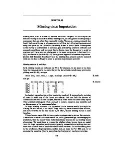
In this paper, for the abalone dataset, the last attribute Rings is set to target attribute, others are set to factor attributes. The experimental results on abalone are presented in Figure 1, from (1) to (6). For the housing dataset, the attribute MEDV is set to target attribute, the results are presented in Figure 2, from (7) to (12). In these figures, ‘Mean substitution’ means the method of imputing missing values with mean, our method is regard as ‘CMI’. In particular, it is the method in [20] while k=1 in our method, i.e., it is the method for missing values imputation without cluster. CMI Meansubstitution

0.025 0.020 0.015 0.010 0.005 0

10

20

30

40

50

k:Number of Clusters

k:Number of Clusters

(2) Missing rate=5%

(1) Missing rate=5%

AE for Variance

0.10 CMI Mean substitution

0.09 0.08 0.07 0.06 0.05 0.04

0

10

20

30

40

50

AE for Distribution Function

0.11 0.10 CMI Mean substitution

0.08 0.06 0.04 0.02 0.00 0

k:Number of Clusters

(3) Missing rate = 20%

0.16 0.14 0.12 0.10 0

10

20

30

40

50

k: Number of Clusters

(5) Missing rate = 40%

AE for Distribution Function

CMI Mean substitution

0.18

30

40

50

CMI Mean substitution

0.25

0.20 AE for Variance

20

(4) Missing rate = 20%

0.22

0.08

10

k:Number of CLusters

0.20 0.15 0.10 0.05 0.00 0

10

20

30

40

50

k:Number of Clusters

(6) Missing rate = 40%

Fig. 1. CMI vs Mean substitution under different missing rates on dataset abalone for variance and distribution function.

AE for Variance

0.042

CMI Mean substitution

0.041 0.040 0.039 0.038 0.037 0.036 0

5

10

15

20

AE for Distribution Function

0.043

0.035 0.030 0.025

CMI Mean substitution

0.020 0.015 0.010 0.005 0.000 0

5

AE for Variance

CMI Mean substitution

0.090 0.085 0.080 0.075 0.070 0.065

0.20 0.18 0.16 0.14 0.12 0.10 0.08 0.06 0.04 0.02 0.00

20

CMI Mean substitution

0 2

0 2 4 6 8 10 12 14 16 18 20 22

4

6 8 10 12 14 1 6 18 20 2 2 k: Number of Clusters

k: Number of Clusters

(10) Missing rate = 20%

(9) Missing rate = 20%

0.20 0.18 0.16 CMI Mean substitution

0.14 0

5

10

15

20

k: Number of Clusters

(11) Missing rate = 40%

AE for Distribution Function

0.40

0.22 AE for Variance

15

(8) Missing rate=5%

AE for Distribution Function

(7) Missing rate=5%

0.100 0.095

10

k:Number of Clusters

k:Number of CLusters

0.35

CMI Mean substitution

0.30 0.25 0.20 0.15 0.10 0.05 0

5

10

15

20

k:Number of Clusters

(12) Missing rate = 40%

Fig. 2. CMI vs Mean substitution under different missing rates on dataset housing for variance and distribution function.

From above figures, the method ‘Mean substitution’ is worst, the kernel method without clustering (k=1 in our CMI algorithm) outperform the former, and we can see that the clustering-based kernel method performs better most of the time than the kernel method that without clustering (i.e., the situation of k=1 when using k-means) in terms of variance and distribution function. All of results of our method are better

than the results of the method ‘Mean substitution’. What’s more, with increase of cluster number k, the average errors (AE) for variance and distribution function are decreasing. That implies that it is reasonable for us to impute missing values with cluster-based kernel methods. Yet the value of AE will increase when the number of clusters is big enough, this trend will be observed in the above figures. That is to say, the more clusters the worse performance the results of imputation are. That is because there will be less instances for imputing missing values in one cluster while the number of clusters become bigger. In our experiments, for the Abalone dataset (in figure 1, (1) to (6)), the best K, that is the number of clusters for K-means algorithm, ranges from 25 to 35; while for the Housing dataset (in figure 2, (7) to (12)), the best K ranges from 4 to 7. Note that for the large dataset, such as, the dataset abalone in Fig.1, the AE increases gradually while in small dataset (for instance, the dataset Housing in Fig.2) it increases rapidly. Because the number of instances in each cluster will change slightly when the dataset is large and there are more observed information for imputing missing values in one cluster. That makes the values of AE for variance and distribution function relatively stable compared with the previous imputation results. These results are consistent with the results obtained by using the G-means algorithm in [19]. This means that user can use the G-means algorithm to work out the number of clusters, i.e. K, for the dataset at first, and then utilizes our CMI algorithm based on the K, in order to deal with the missing value problems on each of the cluster. As a consequence, user will be easily to choose an appropriate K for clustering in advance, without degrading the system performances for missing value imputation.

5. Conclusions and Future Work In this paper, we propose a clustering-based non-parametric kernel-based imputation method, called CMI, for dealing with missing values, which is presented in target attribute in data preprocessing. Extensive experimental results have demonstrated the effectiveness of CMI method in making inference for variance and the distribution function after clustering. In practice, datasets usually present missing values in conditional attributes and class attributes, which makes the problem of missing value imputation more sophisticated. In our future work, we will deal with this problem.

References 1. 2.

3.

Zhang, S.C., et al., (2004). Information Enhancement for Data Mining. IEEE Intelligent Systems, 2004, Vol. 19(2): 12-13. Zhang, S.C., et al., (2005). “M issing is useful”: M issing values in cost-sensitive decision trees. IEEE Transactions on Knowledge and Data Engineering, 2005, Vol. 17(12): 16891693. Qin, Y.S., et al. (2007). Semi-parametric Optimization for Missing Data Imputation. Applied Intelligence, 2007, 27(1): 79-88.

4. 5. 6. 7. 8. 9.

10.

11.

12. 13. 14.

15. 16. 17. 18. 19. 20. 21. 22. 23. 24. 25. 26.

Zhang, C.Q., et al., (2007). An Imputation Method for Missing Values. PAKDD, LNAI 4426, 2007: 1080–1087. Quinlan, J.R. (1993). C4.5: Programs for Machine Learning. Morgan Kaufmann, San Mateo, USA, 1993. Han, J., and Kamber, M., (2006). Data Mining: Concepts and Techniques. Morgan Kaufmann Publishers, 2006, 2nd edition. Chen, J., and Shao, J., (2001). Jackknife variance estimation for nearest-neighbor imputation. J. Amer. Statist. Assoc. 2001, Vol.96: 260-269. Lall, U., and Sharma, A., (1996). A nearest-neighbor bootstrap for resampling hydrologic time series. Water Resource. Res. 2001, Vol.32: 679–693. Chen, S.M., and Chen, H.H., (2000). Estimating null values in the distributed relational databases environments. Cybernetics and Systems: An International Journal. 2000, Vol.31: 851-871. Chen, S.M ., and Huang, C.M ., (2003). Generating weighted fuzzy rules from relational database systems for estimating null values using genetic algorithms. IEEE Transactions on Fuzzy Systems. 2003, Vol.11: 495-506. Magnani, M., (2004). Techniques for dealing with missing data in knowledge discovery tasks. Available from http://magnanim.web.cs.unibo.it/data/pdf/missingdata.pdf, Version of June 2004. Kahl, F., et al., (2001). Minimal Projective Reconstruction Including Missing Data. IEEE Trans. Pattern Anal. Mach. Intell., 2001, Vol. 23(4): 418-424. Gessert, G., (1991). Handling Missing Data by Using Stored Truth Values. SIGMOD Record, 2001, Vol. 20(3): 30-42. Pesonen, E., et al., (1998). Treatment of missing data values in a neural network based decision support system for acute abdominal pain. Artificial Intelligence in Medicine, 1998, Vol. 13(3): 139-146. Ramoni, M. and Sebastiani, P. (2001). Robust Learning with Missing Data. Machine Learning, 2001, Vol. 45(2): 147-170. Pawlak, M., (1993). Kernel classification rules from missing data. IEEE Transactions on Information Theory, 39(3): 979-988. Forgy , E., (1965). Cluster analysis of multivariate data: Efficiency vs. interpretability of classifications. Biometrics, 1965, Vol. 21: 768 Blake, C.L and Merz, C.J (1998). UCI Repository of machine learning databases. Hamerly, H., and Elkan, C., (2003). Learning the k in k-means. Proc. of the 17th intl. Conf. of Neural Information Processing System. Zhang, S.C., et al., (2006). Optimized Parameters for Missing Data Imputation. PRICAI06, 2006: 1010-1016. Wang, Q., and Rao, J., (2002a). Empirical likelihood-based inference in linear models with missing data. Scand. J. Statist., 2002, Vol. 29: 563-576. Wang, Q. and Rao, J. N. K. (2002b). Empirical likelihood-based inference under imputation for missing response data. Ann. Statist., 30: 896-924. Silverman, B., (1986). Density Estimation for Statistics and Data Analysis. Chapman and Hall, New York. Friedman, J., et al., (1996). Lazy Decision Trees. Proceedings of the 13th National Conference on Artificial Intelligence, 1996: 717-724. John, S., and Cristianini, N., (2004). Kernel Methods for Pattern Analysis. Cambridge. Lakshminarayan, K., et al., (1996). Imputation of Missing Data Using Machine Learning Techniques. KDD-1996: 140-145.