Mobile Agent-Based Directed Diffusion in Wireless Sensor Networks

Hindawi Publishing Corporation EURASIP Journal on Advances in Signal Processing Volume 2007, Article ID 36871, 13 pages doi:10.1155/2007/36871

Research Article Mobile Agent-Based Directed Diffusion in Wireless Sensor Networks Min Chen,1 Taekyoung Kwon,2 Yong Yuan,3 Yanghee Choi,2 and Victor C. M. Leung1 1 Department

of Electrical and Computer Engineering, University of British Columbia, Vancouver, BC, Canada V6T 1Z4 of Computer Science and Engineering, Seoul National University, Seoul 151-744, South Korea 3 Department of Electronics and Information Engineering, Huazhong University of Science and Technology, Wuhan 430074, China 2 School

Received 29 November 2005; Revised 12 May 2006; Accepted 16 July 2006 Recommended by Deepa Kundur In the environments where the source nodes are close to one another and generate a lot of sensory data traffic with redundancy, transmitting all sensory data by individual nodes not only wastes the scarce wireless bandwidth, but also consumes a lot of battery energy. Instead of each source node sending sensory data to its sink for aggregation (the so-called client/server computing), Qi et al. in 2003 proposed a mobile agent (MA)-based distributed sensor network (MADSN) for collaborative signal and information processing, which considerably reduces the sensory data traffic and query latency as well. However, MADSN is based on the assumption that the operation of mobile agent is only carried out within one hop in a clustering-based architecture. This paper considers MA in multihop environments and adopts directed diffusion (DD) to dispatch MA. The gradient in DD gives a hint to efficiently forward the MA among target sensors. The mobile agent paradigm in combination with the DD framework is dubbed mobile agent-based directed diffusion (MADD). With appropriate parameters set, extensive simulation shows that MADD exhibits better performance than original DD (in the client/server paradigm) in terms of packet delivery ratio, energy consumption, and end-to-end delivery latency. Copyright © 2007 Min Chen et al. This is an open access article distributed under the Creative Commons Attribution License, which permits unrestricted use, distribution, and reproduction in any medium, provided the original work is properly cited.

1.

INTRODUCTION

Recent years have witnessed a growing interest in deploying a sheer number of microsensors that collaborate in a distributed manner on sensing, data gathering, and processing. In contrast with IP-based communication networks based on global addresses and routing metrics of hop counts, sensor nodes normally lack global addresses. Also, as being unattended after deployment, they are constrained in energy supply (e.g., small battery capacity). These characteristics of sensor networks require energy awareness at most layers of protocol stacks. To address such challenges, most of researches focus on prolonging the network lifetime, allowing scalability for a large number of sensor nodes, or supporting fault tolerance (e.g., sensor’s failure and battery depletion) [2, 3]. Most energy-efficient proposals are based on the traditional client/server computing model, where each sensor node sends its sensory data to a backend processing center or a sink node. Because the link bandwidth of a wireless sensor network is typically much lower than that of a wired network, a sensor network’s data traffic

may exceed the network capacity. To solve the problem of the overwhelming data traffic, Qi et al. [1] proposed the mobile agent-based distributed sensor network (MADSN) for scalable and energy-efficient data aggregation (this aggregation process is called collaborative signal and information processing in [1]). By transmitting the software code, called “mobile agent (MA)” to sensor nodes, the large amount of sensory data can be reduced or transformed into small data by eliminating the redundancy. For example, the sensory data of two closely located sensors are likely to have redundant or common part when the data of two sensors are merged. Therefore, data aggregation is a necessary function in densely populated sensor networks in order to reduce the sensory data traffic. However, MADSN operates based on the following assumptions: (1) the sensor network architecture is clustering based; (2) source nodes are within one hop from a clusterhead; (3) much redundancy exists among the sensory data which can be fused into a single data packet with a fixed size. These assumptions pose much limitation on the range of applications which can be supported by MADSN. This limitation of clustering can be addressed by a flat sensor

2

EURASIP Journal on Advances in Signal Processing

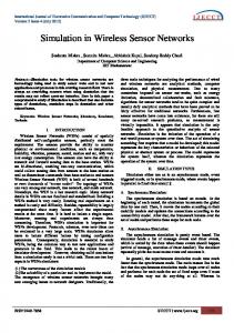
Segment ROI (region of interest) 2 Collect reduced data

3 Migrate to sink node

1 Migrate to target region

Figure 1: Mobile agent-based image sensor querying.

network architecture, which may be suitable for a wide range of sensor applications. Thus, we will consider MA in multihop environments with the absence of a clusterhead. Without clusterhead, we have to answer the following questions. (1) How is an MA routed from sink to source, from source to source, and from source to sink in an efficient way? (2) How does an MA decide a sequence to visit multiple source nodes? (3) If the sensory data of all the source nodes cannot be fused into a single data packet with a fixed size, will the MA paradigm still perform more efficiently than the client/server computing model? How about in the environments where the source nodes are not close to one another, and the sensory data do not have enough redundancy? With the development of WSN, “one-deployment multiple applications” is a trend due to the application-specific nature of sensor networks. Such a trend must require sensor nodes to have various capabilities to handle multiple applications, which is economically infeasible. In general, using memory-constrained embedded sensors to store every possible application in their local memory is impossible. Thus, a way of dynamically deploying a new application is needed. To have an in-depth look at problems we mentioned above and why the MA is necessary, we investigate the following scenario of an image recognition application in wireless sensor networks. In Figure 1, we assume that a number of image sensors are deployed to monitor a remote region. Transmitting the whole pictures taken by individual sensors to a sink node may be overwhelming for the wireless link, or even unnecessary in the case that the sink node needs only the region of interest (ROI) of the picture (e.g., human face or vehicle identification number plate). Thus, instead of transmitting the whole picture, a source node extracts the ROI from the whole picture using an image segmentation algorithm. However, a single kind of image segmentation algorithm cannot achieve fairly good performance for all kinds of images to be extracted. For example, a code for segmenting a face image will be different from the one for segmenting a vehicle identification number plate. However, a sensor network may require various image processing algorithms to

handle different kinds of images of interest. It is impossible to keep all kinds of codes in a sensor node’s limited memory. In order to solve this problem, the sink node can dispatch an MA carrying a specific image segmentation code to the sensors of interest. Carrying a special processing code, the MA enables a source node to perform local processing on the sensed data as requested by the application. When the MA reaches and visits the sensors of interest, the image data at each target sensor node can be reduced into a smaller one by image-segment processing. Since multiple hops may exist among target source nodes, the migration behavior of the MA becomes complicated and it is important to find out a way to dispatch the MA efficiently among the sensors of interest. Directed diffusion (DD) [4, 5] is a prominent example of data-centric routing based on application layer context and local interactions. The gradient in DD gives a hint to efficiently forward the MA among target sensors. The MA paradigm in combination with the DD framework is dubbed mobile agent-based directed diffusion (MADD). This paper investigates this combination: is it feasible to conduct DD with the mobile agent paradigm? How does MA operate in detail? In which condition does MADD outperform DD in terms of energy consumption and endto-end delay? This study also provides insights into the behavior of MA in multihop wireless environments, contributing to a better understanding of this novel combination of mobile agent paradigm and a holistic DD framework. Extensive simulation-based comparison between original DD and MADD shows that, depending on the parameters, MADD can significantly reduce the energy consumption and endto-end delay. The rest of this paper is organized as follows. Section 2 presents related work. We describe MADD design issues and algorithm in Sections 3 and 4, respectively. Simulation model and results are explained in Sections 5 and 6, respectively. Finally, Section 7 will conclude the paper. 2.

RELATED WORK

Recently, mobile agents have been proposed for efficient data dissemination in sensor networks [1, 6–12]. In a typical client/server-based sensor network, the occurrence of certain events will alert sensors to collect data and send them to a sink node. However, the introduction of a mobile agent (MA) leads to a new computing paradigm, which is in contrast to the traditional client/server-based computing. The MA is a special kind of software which visits the network either periodically or on demand (when the application requires). It performs data processing autonomously while migrating from node to node. Although there are advantages and disadvantages (code caching, safety, and security) of using MAs [3] in a particular scenario, their successful applications range from e-commerce [6] to military situation awareness [7]. They are found to be particularly useful for data fusion tasks in distributed sensor networks. The motivations for using MAs in distributed sensor networks have been extensively studied in [1]. As mentioned in Section 1, this paper will adopt DD for routing MA. DD [4] is a data-centric dissemination protocol

Min Chen et al. for sensor networks. It provides the following mechanisms: (a) for a sink node to flood a query toward the sensors of interest (say, sensors detecting event), (b) for intermediate nodes to set up gradients to send data along the routes toward the sink node. DD provides high quality paths, but requires an initial flood of the query to explore paths. In DD, the publish/subscribe mechanism provides a sensor network with application context by attribute-based naming. Attribute-based naming specifies which sensors are responsible for responding queries, and how intermediate sensors perform in network processing. Attributes describe the data which a sink node desires, by specifying sensor types, desired data rate, and possibly some geographical region. A monitoring node becomes a sink, creating attributes of interest specifying a particular kind of data. The interest is propagated over the network towards sensor nodes in the specified region. A key feature of DD is that every sensor node can be application-aware, which means that nodes store and interpret interests, rather than simply forwarding them along. Each sensor node that receives an interest maintains a table that contains which neighbor(s) sent that interest. To such a neighbor, it sets up a gradient. A gradient is used to evaluate the eligibility of a neighbor node as a next hop node for data dissemination. After setting up a gradient, the sensor node redistributes the interest by broadcasting the interest. As interests travel across the network, sensors that match interests are triggered and the application activates its local sensors to begin collecting and sending data. 3.

OVERVIEW OF THE MADD DESIGN

In this section, we discuss the key design issues of MADD. Before describing them, we first present our assumptions about MADD and its applications. (1) Compared with the distance to the sink node, the target sensor nodes are geographically close to each other. (2) Only source nodes matching interest packets will store the processing code carried by an MA. The sink does not flood processing code to the whole network, since the associated communication overhead may be too high. For example, shipping a mobile agent with face detection code would incur an overhead of over 1 MB. However, most of the sensor nodes may not be queried by this application at all. (3) Processing code is stored in the source node when the MA visits it at the first time. The processing code will be operating until the task is scheduled to finish. It may be discarded when the task is finished. (4) The locally processed data in each source node will be aggregated into the accumulated data result of the MA by a certain aggregation ratio. 3.1. Application redundancy eliminating by MA-assisted local processing As described in Section 1, due to the application-specific nature of sensor networks, a sensor should have various capabilities to handle multiple applications. However, it is

3 unrealistic for a memory-constrained embedded sensor to store every possible application code in its local memory. The introduction of MA not only provides an efficient way of dynamically deploying a new application, but also allows a source node to perform local processing on the raw data as requested by the application. This capability enables a reduction in the amount of data to be transmitted since only relevant information will be extracted and transmitted. Let r (0 < r < 1) be the reduction ratio by the MA-assisted local processing, let Sidata be the size of raw data at source i, and let Ri be the size of reduced data. Then, Ri = Sidata · (1 − r). 3.2.

(1)

Aggregation

The degree of sensed data correlation among sensors is closely related to the distance between sensors so that it is very likely for closely located sensors to generate redundant sensed data. Therefore, data aggregation, which eliminates unnecessary data transmissions, is a necessary function in densely populated sensor networks in order to refine the sensed data as well as to extend the network lifetime. Because the aggregation decisions are made as the data is disseminated in the network, this is also referred to as in-network processing. In DD, different data packets which are completely/ partially redundant each other are forwarded to the sink through multiple paths with a low probability to be aggregated. This aggregation technique can be considered as opportunistic aggregation. In contrast, the MA aggregates individual sensed data when it visits each target source. Though this kind of aggregation technique is typically used in clustering or aggregation tree-based data dissemination protocols, the aggregation in MADD does not need any overhead to construct these special structures. Note that MADD builds the gradient for routing as DD does, and does not need more control overhead than DD. We calculate the size of data result accumulated by the MA using the similar method in [9]. A sequence of data result can be fused with an aggregation ratio (ρ, 0 ≤ ρ ≤ 1). Let Sima be the amount of accumulated data result after the MA leaves source i, where Ri is the amount of data that will be aggregated by ρ. Then, S1ma = R1 , S2ma = R1 + (1 − ρ) · R2 .. . i−1 Sima = Sma + (1 − ρ) · Ri

= R1 +

i 

(2)

(1 − ρ) · Rk .

k=2

In (2), there is no data aggregation in the first source. The value of ρ is dependent on the type of application. For the image processing application described in Section 1, when we fuse two ROI images, effective data fusion can be attained

4

EURASIP Journal on Advances in Signal Processing Data collection is finished at the last source

8 7

6 1 5 2 4

3

Intermediate node Source node Sink node

Target region Mobile agent

Figure 2: Gradient-based solution for deciding the order of source nodes to be visited.

only if statistical characteristics of the image are known (e.g., Slepian-Wolf coding schemes [13]), which implies that data aggregation may not be achieved efficiently. By comparison, the application considered in [1] is an extreme example, where the sensory data can be fused into a data with fixed size (say, ρ = 1). 3.3. Efficient routing The order of source nodes to be visited by the MA can have a significant impact on energy consumption. Finding an optimal source-visiting sequence is an NP-complete problem. In [10], a genetic algorithm-based solution to compute an approximate solution is presented. Though global optimization can be achieved using genetic algorithm, it is not a lightweight solution for sensor nodes that are constrained in energy supply. This paper adopts a gradient-based solution (in Section 4.3) for the MA to dynamically decide the route. Figure 2 gives an example of deciding source-visiting sequence through the gradient-based solution. 4.

to the sink individually. Then, the sink will receive these exploratory data packets from various sources and decide the list of sources that will be visited by an MA. In the list, there are two sources whose positions are important, namely, the first source which the MA will visit (FirstSrc) and the last source (LastSrc). The MA-related operation begins at the point of the sink dispatching MA and ends when the MA returns to the sink with collected results. The whole route can be generally divided into three parts demarcated by FirstSrc and LastSrc (i.e., from the sink to FirstSrc, from FirstSrc to LastSrc, and from LastSrc to the sink). In most cases, each source is expected to generate the sensory data periodically with some interval, which means the same code (MA) needs to be stored for multiple runnings. Thus, when the MA arrives at the FirstSrc, it will be stored. Then, FirstSrc sets a Create-MA-Timer, which is used to trigger the next round to dispatch the MA to collect data from the relevant sources again. Obviously, the interval between the successive rounds will be equal to the sensory data generating rate which is set to the value of the Create-MA-Timer. This round will be repeated until the task is finished. A round can also be defined as the interval from the time that an MA collects the data packet in the FirstSrc to the time that it collects the data packet in LastSrc. At the end of the last round, the task is finished. When the Create-MA-Timer expires, FirstSrc starts a new round by dispatching the MA along all the sensors. After an MA visits the LastSrc, it discards the processing code and carries the aggregated result to the sink. The sink will be expected to receive an MA by the desired data rate until the task is finished. Based on the above illustration, the differences between MADD and client/server-based WSN can be listed as follows. (1) All the relevant sources in client/server-based WSN send sensory data individually with a specified interval; while in MADD, a single MA visiting all the relevant sources will collect the data. The interval between reports to the sink is decided by the dispatching rate of the MA. (2) In client/server-based WSN, data results are sent back in parallel from all sources, or return to the sink; while in MADD, data is collected by the MAs visiting all the target sensors along a single path.

THE MADD ALGORITHM 4.2.

Section 4.1 gives an overview of the algorithm. Section 4.2 describes the structure of the MADD packet. Section 4.3 illustrates MADD with the details. Then, we give a simple performance analysis in Section 4.4 4.1. Algorithm overview The flowchart of the MADD protocol is shown in Figure 3. Once receiving a new task as requested by an application, the sink initially floods an interest packet to find out the sources which will perform the task. If the sources in the target region receive the interest packets, they flood exploratory data

Mobile agent packet format

The information contained in an MA packet is shown in Figure 4. The pair of SinkID and MA SeqNum is used to identify an MA packet. Whenever a sink dispatches a new MA packet, it will increment the MA SeqNum. FirstSrc and LastSrc are the source nodes scheduled to be visited firstly and lastly by the MA, respectively. The pair of FirstSrc and LastSrc indicates the beginning and ending points of MA’s data gathering. RoundIdx is the index of current round. The value is initially set to 1 by the sink in the first round, and will be incremented by the FirstSrc in the following rounds. LastRoundFlag indicates that the current round is the last round

Min Chen et al.

5 Idle state

Receive new task (I am a sink)

A A

Receive interset (I am a source)

B

Receive E-datas sent by n sources (I am the sink)

C

Visited by MA (I am FirstSrc)

D

Expire Create-MA-Timer (I am FirstSrc)

E

Visited by MA (I am non-FirstSrc)

Flood interest Flood exploratory data (E-data) Set FirstSrc and SrcList to the MA

Create MA

Dispatch MA

Start Create-MA-Timer

Store the MA

No

Create MA by copying the stored one

Last round?

Am I the LastSrc in the SrcList?

Yes

No

Yes

MA collects data and migrates to NextSrc in the SrcList

MA collects data and migrates to the sink

Figure 3: Flowchart of the basic MADD protocol.

Fixed attributes SinkID MA SeqNum FirstSrc LastSrc RoundIdx LastRoundFlag Variable attributes NextSrc

NextHop

ToSinkFlag

SrcList

Payload Processing code

Data

Figure 4: MA packet structure.

of the whole task. The flag is set by FirstSrc. When an MA with LastRoundFlag set arrives at a source node, it can make the system unmount the corresponding processing code after its execution. When an MA migrates, it may change variable attributes. NextSrc specifies the next destination source node to be visited. NextHop indicates the immediate next hop node which is an intermediate sensor node or a target source node. If NextHop is equal to NextSrc, it means that the next hop node is current destination source. SrcList contains the identifiers (IDs) of target sensor nodes that remain to be visited in the current round. It does not contain any information of source-visiting sequence since NextSrc is dynamically decided when an MA arrives at a source node (except LastSrc). SrcList initially contains all the IDs of source nodes when an MA is created. The corresponding ID will be deleted after the MA visits the source node. If all the target sources have been

visited by the MA, ToSinkFlag is set to indicate that the destination of the MA is the sink. NextSrc, NextHop, SrcList, and ToSinkFlag hint the dynamical route of MA migration. Payload includes two kinds of data. One is ProcessingCode which is used to process sensed data; the other is Data which carries the accumulated data result. The size of Data is zero when an MA is generated, and increases while the MA migrates from source to source. 4.3.

Detailed illustration of MADD protocol and gradient-based MA routing

The proposed MADD mechanism is based on the original DD (two-phase pull DD). In this DD, the sink initially diffuses an interest for notifications of low-rate exploratory events which are intended for path setup and repair. The gradients set up for exploratory events are called exploratory gradients. The multiple exploratory gradients can enable fast recovery from failed paths or reinforcement of empirically better paths. Once target sources receive the corresponding interest, they send exploratory data, possibly along multiple paths, toward the sink. The initial flooding of the interest, together with the flood of the exploratory data, constitutes the first phase of two-phase pull DD. If the sink has multiple previous hop nodes, it chooses a preferred neighbor to receive subsequent data messages for the same interest (e.g., the one which delivered the exploratory data earliest). To do this, the sink reinforces the preferred neighbor, which in turn, reinforces its preferred previous hop node, and so on. Periodically, the source sends additional exploratory data

6

EURASIP Journal on Advances in Signal Processing

A

B 15

14

C 16

13

17

D

12 10

9

6

11 7

8

5 4

2 1

3 E Sink

Sink node Intermediate node First source node Last source node

Positive reinforcement Mobile agent migrates toward event region Mobile agent migrates among source nodes Mobile agent migrates along reinforced path

Intermediate source node

Figure 5: Second phase of MADD.

messages to adjust gradients in the case of network changes (due to node failure, energy depletion, or mobility), temporary network partitions, or to recover from lost exploratory messages. The path reinforcement and the subsequent transmission of data along reinforced paths constitute the second phase of two-phase pull DD. The first phase of MADD is identical to that of DD, however, in addition to path reinforcement, in the second phase, an MA is sent to target source nodes matching the sink’s interests. Figure 5 depicts the detailed operation of the second phase in the MADD scheme. At the end of the first phase, the target sensor nodes generate multiple exploratory message flows to the sink. Since the ultimate goal is the detection of events in sensor networks [14], the sink may stop handling any exploratory message flows if it considers that the number of source nodes is large enough to meet the requirement of reliable event detection. Thus all the source nodes or only a subset of these nodes will be chosen to be visited by MA. Among the target source nodes to be visited, the sink will choose the first and last source nodes. Then, the sink generates an MA with the packet format described in Figure 4, and dispatches it to the first source. At the same time, the sink reinforces the path to the last source. When the MA arrives at the first source node, it is stored in the node. We divide the whole task period into rounds, where each round requires the MA to visit all the chosen target sensors and to return the data result to the sink. The MA starts from the first

source (or from the sink only in the first round) and arrives at the last source. Finally, the MA will carry the data result to the sink along the reinforced path. In the first round, in addition to that the MA moves from source to source to collect and aggregate information, it also copies processing code into the memory of each source node. At the beginning of each round, the first source node will construct another MA from its memory and dispatch it to initiate the new round. Since processing code has already resided in each source node after the first round, the MA does not carry the processing code any more in the following rounds. When the whole task is finished, all the source nodes will discard the processing code. In the first phase of MADD, the initial flooding of the interest enables each sensor node (e.g., intermediate sensor node or source node) to set up exploratory gradients [15] which are used to deliver exploratory messages intended for path setup and repair. The exploratory gradients, which are denoted as exp., are shown in Figure 6(a). After path reinforcement, the updated gradients are shown in Figure 6(b). The gradient to deliver MA is denoted by MA. The identifier of each node is equal to the one in Figure 5. In MADD, target source nodes flooding exploratory messages enable sensor nodes to set up ToSourceEntry, which is a kind of gradient toward each target source. ToSourceEntry is used for MA to roam among source nodes. In this paper, a time-to-live (TTL) field is set in exploratory message to mandate only the sensor nodes within the target region to set up their ToSourceEntries. The value of TTL is decreased as exploratory message is propagated hop by hop. If the value is equal to 0, sensor nodes do not set up ToSourceEntry any more. Among all the neighbors of a sensor node, only the neighbor who first relays the exploratory message of a specific target source will be chosen as the sensor node’s NextHop in the ToSourceEntry. In Figure 5, nodes A, B, C, and D are the target source nodes. The ToSourceEntries set up by nodes A, B, C, 16, and D are shown in Figure 7. Based on the gradients and ToSourceEntries, a migrating route is decided by the following three operating elements. (1) Choose FirstSrc and LastSrc. According to (2), the size of an MA is the minimum in FirstSrc while it becomes the maximum in LastSrc. Thus, to reduce total communication overhead, FirstSrc should be the farthest target sensor from the sink, while LastSrc should be the closest one. In this paper, the target source which is the last (first) to send exploratory messages to the sink is chosen as FirstSrc (LastSrc). The sink will reinforce the path to LastSrc. (2) Decide source-visiting sequence. Except that FirstSrc and LastSrc are chosen by the sink, the sequence of visiting the other source nodes is dynamically decided by each target sensor in SrcList. For example, when an MA arrives at node A in Figure 5, the node will choose the closest next source node based on its ToSourceEntry shown in the first row of Figure 7. Since the lowest latency of node B is the least, it implies that node B is the closest source node from node A and is chosen as NextSrc.

Min Chen et al.

7 4.4.

Gradient (interest SeqNum = 1) D

Direction type

7 exp.

10 exp.

13 exp.

16 exp.

17 exp.

11 exp.

7

Direction type

5 exp.

6 exp.

10 exp.

D exp.

11 exp.

8 exp.

5

Direction type

4 exp.

6 exp.

7 exp.

8 exp.

2 exp.

1 exp.

2

Direction type

E exp.

1 exp.

5 exp.

3 exp.

— —

— —

(a)

Gradient (interest SeqNum = 1) D

Direction type

7 MA

10 exp.

13 exp.

16 exp.

17 exp.

11 exp.

7

Direction type

5 MA

6 exp.

10 exp.

D exp.

11 exp.

8 exp.

5

Direction type

4 exp.

6 exp.

7 exp.

8 exp.

2 MA

1 exp.

2

Direction type

E MA

1 exp.

5 exp.

3 exp.

— —

— —

(b)

Figure 6: Gradients to the sink. (a) Before reinforcement. (b) After reinforcement.

Performance analysis

In this section, we present a simple analysis that evaluates the key performance metrics of DD and MADD, including the average end-to-end delay for a data packet delivery (Tete ) and the cumulative energy consumption involved in forwarding data packets from all the source nodes to the sink in one round(E). Let Tdd and Tma denote Tete of DD and MADD, respectively. It accounts for all possible delays during data dissemination, caused by queuing, retransmission due to collision at the MAC, and transmission time. Let H be the number of hops along the path between LastSrc and the sink, which is actually the lowest latency path among all the source-sink pairs. Let H + h be the average number of hops of all the source-sink pairs in DD. Sdata is the size of sensed data and Sh is the size of packet header. Let vn be the data rate at MAC layer; let tctrl be the total delay for control messages (say, ACK) during a successful data transmission. In DD, multiple data results sent in parallel from all sources are likely to contend for the channel (CSMA-CA) and potentially collide, which causes additional delay for data retransmissions, especially as the number of source nodes becomes large. Let taccess be the average latency to transmit a data packet successfully in DD. Let Tr be the average latency for path reinforcement. Let ndata be the number of data packets delivered to the sink during the task. Then, Tdd is equal to 

ToSourceEntry (exploratory message SeqNum = 5) Source

A

B

C

D

A

NextHop Lowest Latency (ms)

— —

B 4.46

B 8.24

14 16.32

B

NextHop Lowest Latency (ms)

A 4.47

— —

C 4.43

C 12.89

C

NextHop Lowest Latency (ms)

B 8.16

B 4.32

— —

16 8.52

16

NextHop Lowest Latency (ms)

15 9.65

C 7.56

C 4.86

D 5.08

D

NextHop Lowest Latency (ms)

10 14.15

16 12.67

16 8.73

— —



Tr S + Sh + data + tctrl + taccess · (H + h) ndata vn   Sdata + Sh ≈ + tctrl + taccess · (H + h) vn   if ndata  1 .

Tdd =

In MADD, Tma is the average time interval between the time an MA is created and the time the MA returns to the sink. Let T p be the delay of the MA migrating from the sink to the FirstSrc; let Troam be the average latency of MA roaming from the FirstSrc to the LastSrc; let Tback be the average delay of MA migrating from the LastSrc to the sink. Let τ be the MA accessing delay (e.g., the time for an MA to amount processing code in target source). Let S p be the size of processing code; let v p be the data processing rate; let Sima be the size of MA at source i; let N be the number of source nodes. Then, Troam is equal to

Figure 7: ToSourceEntry setup after exploratory messages flooding.

Troam =

N  

τ+

i=1

(3) Find the next hop node to route an MA along the entire path from sink to source, source to source, and source to sink. Dispatched by the sink, an MA migrates to FirstSrc in the same manner as a reinforcement message is forwarded in original DD. When the MA migrates among target sources, its next hop node will be decided according to current node’s ToSourceEntry. The MA will return to the sink using the reinforced path (e.g., path D-7-5-2-E in Figure 5).

(3)



Sdata Sima + S p + Sh + + tctrl . vp vn

(4)

In (4), Sima is equal to 

 



i−1 Sima = Sma + Sdata · 1 − ri · 1 − pi .

(5)

Let SNma be the size of an MA packet after the MA visits LastSrc. Then, Tback is equal to Tback =





SNma + Sh + tctrl · H. vn

(6)

8

EURASIP Journal on Advances in Signal Processing Then, Tma can be calculated as follows:

Sensor nodes Sink

Tp + Troam + Tback ndata   ≈ Troam + Tback if ndata  1 .

Tma =

Target region

(7)

Let Edd and Ema denote E of DD and MADD, respectively. Let mtx and mrx be the energy consumption for receiving and transmitting a bit, respectively. Let b be the fix energy cost to transmit a packet. Let ectrl be the energy consumption of control messages exchanged for a successful data transmission. Let eretx be the energy consumption of packet retransmissions for a successful data transmission in case of congestion in DD. Then, Edd is equal to Edd =



 

Sdata + Sh · mtx + mrx





+ b + ectrl + eretx · (H + h) · N.

(8) Figure 8: Sensor network model.

In MADD, let E p be the energy consumption of MA migrating from the sink to the FirstSrc; let Eroam be the average energy consumption of MA roaming from the FirstSrc to LastSrc; let Eback be the average energy consumption of MA migrating from the LastSrc to the sink. Let m p be the energy consumption for processing a bit. Then, Eroam is equal to Eroam =

N   i=1



Sdata · m p + Sima + S p + Sh

Application layer Sensor App manager



   · mtx + mrx + b + tctrl .

(9)

MADD routing

Routing layer MADD and directed diffusion routing

Wlan mac intf

Data link layer IEEE 802.11 implementation + interface

Eback is equal to Eback =

 







SNma + Sh · mtx + mrx + b + tctrl · H.

(10)

Finally, Ema can be calculated as follows: Ep + Eroam + Eback ndata   ≈ Eroam + Eback if ndata  1 .

Ema =

5.

1. Sensor module: constant bit rate (CBR) real-time & best-effort traffic generator 2. App manager module: application-specific in-network processing

Wirless lan mac

Physical layer WLAN receiver (rx) + WLAN transmitter (tx)

Wlan port rx 0 Wlan port tx 0

Figure 9: Sensor node model.

(11)

THE SIMULATION MODEL

5.1. Simulation settings In order to demonstrate the performance of MADD, we choose a client/server-based scheme (i.e., DD) to compare with MADD. We use OPNET [16, 17] for discrete event simulation. Figure 8 illustrates our sensor network. Figure 9 shows the protocol stack of our sensor node model; it includes application layer, routing layer, data link layer, and physical layer. Each task requires periodic transmission of data packets with a constant bit rate (CBR) of 1 packet/s. The sensor nodes are battery operated except the sink. The sink is assumed to have infinite energy supply. We assume that both the sink and sensor nodes are stationary. The sink is located close to one corner of the area, while the target sensor nodes are specified at the other corner. We use the energy model in [18]. The energy consumption parameters are shown in

Table 1. Every node starts with the same initial energy budget (4,500 W·s) [18]. We use the following equation to calculate the energy consumption in three states (transmitting, receiving, or overhearing): m × PacketSizeMAC + b + Pidle × t × 1000 (μW · s).

(12)

Note that to express power consumption in idle state, Pidle , in μW unit, 1000 is multiplied. In (12), m represents the incremental cost compared to the power consumption in idle state, b represents the fixed cost independent of the packet size, t represents the duration of the state, and PacketSizeMAC represents the size of the MAC packet. The parameter values used in the simulations are presented in Table 2. The basic settings are common to all the experiments. For each experiment, we simulate for sixty times with different random seeds and get the average results.

Min Chen et al.

9

Table 1: Energy consumption parameters configuration of lucent IEEE802.11 WaveLAN card [17]. Normalized initial energy of sensor node (W·sec) Incremental cost (μW·s/bytes)

Fixed cost (μW·s)

4500

mtx

1.9

mrecv moverhearing

0.5 0.39

btx

454

brecv

356 140

boverhearing Pidle (mW)

843 Table 2: Simulation setting. Basic specification

Network size Topology configuration mode Total sensor node number Data rate at MAC layer (vn ) Transmission range of sensor node Long retry limit Short retry limit

transmitting, receiving, and overhearing during simulation. Recall that ndata denotes the number of data packets delivered to the sink. Then, e is equal to

500 m × 500 m Randomized 1500 1 Mbps 60 m

e=

Number of source nodes (N)

η= 6.

Default: 5

Size of sensed data (Sdata ) Size of control message

Default: 1 KB Default: 128 B

Sensed data packet interval Duration

Default: 1 s Default: 300 s

MADD specification Raw data reduction ratio (r) in (1) Aggregation ratio (ρ) in (2) MA accessing delay (τ) in (4) Data processing rate (v p ) in (4) Size of processing code (Sproc )

Default: 0.8 Default: 0.2 Default: 10 ms Default: 50 Mbps Default: 2 MB

5.2. Performance metrics In this section, five performance metrics are evaluated. (i) Reliability (packet delivery ratio). It is denoted by P. It is the ratio of the number of data packets delivered to the sink to the number of packets generated by the source nodes. (ii) Energy consumption per successful data delivery. It is denoted by e. It is the ratio of network energy consumption to the number of data packets successfully delivered to the sink. The network energy consumption includes all the energy consumption by transmitting and receiving during simulation. As in [1], we do not account energy consumption for idle state, since this part is approximately the same for all the schemes simulated. Let Etotal be all the energy consumption by

(13)

(iii) Average end-to-end packet delay. It is denoted by Tete . And we also use Tdd and Tma to denote the average end-to-end delays in DD and MADD, respectively. It includes all possible delays during data dissemination, caused by queuing, retransmission due to collision at the MAC, and transmission time. (iv) Energy∗ delay/reliability. In sensor networks, it is important to consider both energy and delay. In [19], the combined energy∗ delay metric can reflect both the energy usage and the end-to-end delay. Furthermore, in unreliable environment, the reliability is also an important metric. In this paper, we adopt the following metric to evaluate the integrated performance of reliability, energy, and delay:

Default: 4 Default: 7 Sensed traffic specification

Etotal . ndata

e · Tete . P

(14)

PERFORMANCE EVALUATION

In this section, we compare the above performance metrics of DD and MADD, and determine the conditions under which MADD is more efficient than DD by simulation. Though these conditions are affected by many parameters, only a set of important parameters is chosen, such as the duration of the task (Ttask ), reduction ratio (r), aggregation ratio (ρ), size of sensed data of each sensor (Sdata ). If we set ρ to 0, it means that data aggregation does not work, all the reduced sensed data are concatenated. When MADD is applied to a wide range of applications, the consideration of varying both r and ρ is necessary. In the image processing application described in Section 1, if the target camera sensors are sparsely distributed, the redundancy between two ROI images is low, which implies that the value of ρ would be small (e.g., ρ = 0.2). In the following sections, several groups of simulations are evaluated. Only one parameter (e.g., Ttask , r, ρ, and Sdata ) is changed in each group while the other parameters are fixed. 6.1.

Comparison of MADD and DD with variable duration of task

In these experiments, we change Ttask from 10 seconds to 600 seconds. In Figure 10, e decreases as Ttask increases in both DD and MADD. When the Ttask is small (i.e., lower than 60 seconds), MADD has higher e than DD because MADD consumes energy (E p ) to transmit processing code from the sink to the target region. Note that E p is a fixed value. If Ttask is small, ndata is small, and e is large. However, when Ttask is beyond 90 seconds with r equal to 0.8 and ρ equal to 0.2, MADD has lower e than DD. Thus, to amortize the cost of shipping the

10

EURASIP Journal on Advances in Signal Processing

105

0.45 Average end-to-end packet delay (mW/s)

Energy consumption per successful data delivery (mW/s)

9 8 7 6 5 4 3 2

0.4 0.35 0.3 0.25 0.2 0.15 0.1

1 0.05 0

0

100

200

300 400 Duration (s)

500

0

0.005 0.01 0.015 0.02 0.025 0.03 0.035 0.04 0.045 0.05 Mobile agent access delay (s)

600

Client/server MA r = 0.9 p = 0.1 MA r = 0.8 p = 0.2

Client/server MA r = 0.9 p = 0.1 MA r = 0.8 p = 0.2

Figure 11: The impact of τ on Tete .

Figure 10: The impact of Ttask on e. 1

processing code once to source node, the source should process enough long streams of data.

0.95

In these experiments, we change τ from 0 seconds to 0.05 seconds. In Figure 11, Tdd is constant since changing τ has no effect on DD. Since the delay of τ is introduced when MA visits each source, τ causes Tma increase fast if the value is set to a large value. In Figure 11, when τ is beyond 0.042 seconds with r equal to 0.8 and ρ equal to 0.2, MADD has larger end-to-end delay than DD. The value of τ is dependent on the middleware environments of mobile agent system. 6.3. Comparison of MADD and DD with variable size of sensed data In these experiments, we change the size of sensed data of each sensor (Sdata ) from 0.5 KB to 2 KB by increasing 0.25 KB each time, and keep the other parameters in Table 2 unchanged. For MADD, several groups of simulations are evaluated with variables r and ρ. In Figure 12, MADD always outperforms DD in terms of P. In MADD, only single data flow is sent for each round. In contrast, multiple data flows from individual source nodes are sent in DD. Thus, congestion in DD is more likely to happen than in MADD. When Sdata increases, the congestion is more serious and P of DD will decrease more. In Figure 13, the energy consumption of DD is larger than that of MADD in most cases. The larger is r or ρ, the smaller is e in MADD. When r is equal to 0.9 and ρ is equal to 1, e is lowest among all the simulations, and it is insensitive to

Packet delivery ratio

0.9

6.2. Comparison of MADD and DD with variable MA accessing delay

0.85 0.8 0.75 0.7 0.65 0.6 0.5

1

1.5

2

Sensed data size (KB) Client/server MA r = 0.9 p = 1 MA r = 0.9 p = 0.5 MA r = 0.9 p = 0.2 MA r = 0.8 p = 0.2

MA r MA r MA r MA r

= 0.7 = 0.6 = 0.5 = 0.4

p = 0.2 p = 0.2 p = 0.2 p = 0.2

Figure 12: The impact of Sdata , r, and ρ on P.

the increase of Sdata . If ρ = 1, all the sensory data will be fused into a data with fixed size. We expect that as ρ decreases, the advantages of MADD will decrease. As we take a conservative approach in evaluation, we will set ρ to a small value in most scenarios. Given ρ fixed to 0.2, when r is beyond 0.6, e of MADD is always less than that of DD, and the performance gain of MADD increases as r increases. When r is less than 0.4, MADD tends to have larger e, since the smaller is r, the larger is the size of the accumulated data result.

Min Chen et al.

11

105

2.5

2

2 Energy  delay/reliability

Energy consumption per successful data delivery (mW/s)

105

2.5

1.5

1

1.5

1

0.5

0.5

0 0.5

1

1.5

0 0.5

2

1

Sensed data size (KB) MA r MA r MA r MA r

Client/server MA r = 0.9 p = 1 MA r = 0.9 p = 0.5 MA r = 0.9 p = 0.2 MA r = 0.8 p = 0.2

= 0.7 = 0.6 = 0.5 = 0.4

p = 0.2 p = 0.2 p = 0.2 p = 0.2

Client/server MA r = 0.9 p = 1 MA r = 0.9 p = 0.5 MA r = 0.9 p = 0.2 MA r = 0.8 p = 0.2

Figure 13: The impact of Sdata , r, and ρ on e.

2

MA r MA r MA r MA r

= 0.7 = 0.6 = 0.5 = 0.4

p = 0.2 p = 0.2 p = 0.2 p = 0.2

Figure 15: The impact of Sdata , r, and ρ on η.

possibly in most scenarios. These figures also give hints that MADD should choose r and ρ appropriately. Given ρ fixed, to find the bounds of r in terms of η, Figure 15 is plotted. It can be observed that MADD has no advantage if ρ is equal to 0.2 and r is smaller than 0.4. Note that the value of r and ρ is dependent on the type of application. Before we adopt MADD for data dissemination, the features of the application should be investigated. MADD will be selected if enough high r and/or ρ can be attained.

1 Average end-to-end packet delay (s)

1.5

Sensed data size (KB)

0.9 0.8 0.7 0.6 0.5 0.4 0.3

7.

0.2 0.1 0 0.5

1

1.5

2

Sensed data size (KB) Client/server MA r = 0.9 p = 1 MA r = 0.9 p = 0.5 MA r = 0.9 p = 0.2 MA r = 0.8 p = 0.2

MA r MA r MA r MA r

= 0.7 = 0.6 = 0.5 = 0.4

p = 0.2 p = 0.2 p = 0.2 p = 0.2

Figure 14: The impact of Sdata , r, and ρ on Tete .

In Figure 14, Tma exhibits similar trend as e of MADD. And Tma is more sensitive to Sdata than e. When ρ is equal to 0.2 and r is less than 0.6, MADD tends to have larger end-toend packet delay than DD. In Figures 12, 13, and 14, MADD exhibits more consistent and relatively higher reliability, lower energy consumption than DD by compromising end-to-end delay bound

CONCLUSIONS

Recently, mobile agents have been proposed for efficient data dissemination in sensor networks. In [1], the authors proposed mobile agent-based distributed sensor network (MADSN) for cluster-based sensor networks. MADSN has many advantages (e.g., scalability, extensibility, energy awareness, reliability), and it is more efficient for sensor networks than the client/server architecture. However, MADSN operates based on the following assumptions: (1) the sensor network architecture is clustering based; (2) source nodes are within one hop from a clusterhead; (3) much redundancy exists among the sensory data which can be fused into a single data packet with a fixed size. These assumptions pose much limitation on the range of applications which can be supported by MADSN. This paper investigates a scenario of image processing application over wireless sensor networks, where multiple hops may exist between target source nodes, and the sensory data packets may not be aggregated efficiently. Such applications pose additional challenges of designing a mobile agent-based architecture over sensor network. To address such challenges, this paper proposes a novel combination of mobile agent paradigm and a holistic

12 sensor network architecture—directed diffusion. The combined framework is dubbed mobile agent-based directed diffusion (MADD). On top of DD, a gradient-based routing scheme is proposed for mobile agent to efficiently migrate from sink to source, source to source, and source to sink. We verify the efficacy of MADD by extensive simulations. The simulation results show that the end-to-end delay of MADD is worse than that of DD in certain conditions, but in most cases, the MADD’s performance in terms of energy consumption is better than that of DD. Thus, for the scenarios where energy consumption is of primary concern, MADD exhibits substantially longer network lifetime than DD.

EURASIP Journal on Advances in Signal Processing

[11]

[12]

[13]

[14]

ACKNOWLEDGMENTS This work was supported by Grant no. (R01-2004-00010372-0) from the Basic Research Program of the Korea Science and Engineering Foundation, and was supported in part by the Canadian Natural Sciences and Engineering Research Council under Grant STPGP 322208-05.

[15]

[16] [17]

REFERENCES [1] H. Qi, Y. Xu, and X. Wang, “Mobile-agent-based collaborative signal and information processing in sensor networks,” Proceedings of the IEEE, vol. 91, no. 8, pp. 1172–1183, 2003. [2] J. N. Al-Karaki and A. E. Kamal, “Routing techniques in wireless sensor networks: a survey,” IEEE Wireless Communications, vol. 11, no. 6, pp. 6–28, 2004. [3] K. Akkaya and M. Younis, “A survey on routing protocols for wireless sensor networks,” Ad Hoc Networks, vol. 3, no. 3, pp. 325–349, 2005. [4] C. Intanagonwiwat, R. Govindan, and D. Estrin, “Directed diffusion: a scalable and robust communication paradigm for sensor networks,” in Proceedings of the 6th Annual ACM/IEEE International Conference on Mobile Computing and Networking (MOBICOM ’00), pp. 56–67, Boston, Mass, USA, August 2000. [5] F. Silva, J. Heidemann, R. Govindan, and D. Estrin, “Directed diffusion,” Tech. Rep. ISI-TR-2004-586, USC/Information Sciences Institute, Los Angeles, Calif, USA, January 2004, to appear in Frontiers in Distributed Sensor Networks, S. S. Iyengar and R. R. Brooks, Eds. [6] C. G. Harrison and D. M. Chess, “Mobile agents: are they a good idea?” Tech. Rep. RC 1987, IBM T. J. Watson Research Center, Yorktown Heights, NY, USA, March 1995. [7] P. Dasgupta, N. Narasimhan, L. E. Moser, and P. M. MelliarSmith, “MAgNET: mobile agents for networked electronic trading,” IEEE Transactions on Knowledge and Data Engineering, vol. 11, no. 4, pp. 509–525, 1999. [8] K. N. Ross, R. D. Chaney, G. V. Cybenko, D. J. Burroughs, and A. S. Willsky, “Mobile agents in adaptive hierarchical Bayesian networks for global awareness,” in Proceedings of the IEEE International Conference on Systems, Man and Cybernetics, vol. 3, pp. 2207–2212, San Diego, Calif, USA, October 1998. [9] Y.-C. Tseng, S.-P. Kuo, H.-W. Lee, and C.-F. Huang, “Location tracking in a wireless sensor network by mobile agents and its data fusion strategies,” Computer Journal, vol. 47, no. 4, pp. 448–460, 2004. [10] Q. Wu, N. S. V. Rao, J. Barhen, et al., “On computing mobile agent routes for data fusion in distributed sensor networks,”

[18]

[19]

IEEE Transactions on Knowledge and Data Engineering, vol. 16, no. 6, pp. 740–753, 2004. C.-Y. Chong and S. P. Kumar, “Sensor networks: evolution, opportunities, and challenges,” Proceedings of the IEEE, vol. 91, no. 8, pp. 1247–1256, 2003. M. Chen, T. Kwon, and Y. Choi, “Data dissemination based on mobile agent in wireless sensor networks,” in Proceedings of 30th Annual IEEE Conference on Local Computer Networks (LCN ’05), pp. 527–529, Sydney, Australia, November 2005. J. Bajcsy and P. Mitran, “Coding for the Slepian-Wolf problem with turbo codes,” in Conference Record / IEEE Global Telecommunications Conference (GLOBECOM ’01), vol. 2, pp. 1400– 1404, San Antonio, Tex, USA, November 2001. ¨ B. Akan, and I. F. Akyildiz, “ESRT: Y. Sankarasubramaniam, O. event-to-sink reliable transport in wireless sensor networks,” in Proceedings of the International Symposium on Mobile Ad Hoc Networking and Computing (MobiHoc ’03), pp. 177–188, Annapolis, Md, USA, June 2003. F. Zhao, J. Shin, and J. Reich, “Information-driven dynamic sensor collaboration,” IEEE Signal Processing Magazine, vol. 19, no. 2, pp. 61–72, 2002. http://www.opnet.com. M. Chen, OPNET Network Simulation, Tsinghua University Press, Beijing, China, 2004. L. M. Feeney and M. Nilsson, “Investigating the energy consumption of a wireless network interface in an ad hoc networking environment,” in Proceedings of 20th Annual Joint Conference of the IEEE Computer and Communications Societies (INFOCOM ’01), vol. 3, pp. 1548–1557, Anchorage, Alaska, USA, April 2001. S. Lindsey, C. Raghavendra, and K. M. Sivalingam, “Data gathering algorithms in sensor networks using energy metrics,” IEEE Transactions on Parallel and Distributed Systems, vol. 13, no. 9, pp. 924–935, 2002.

Min Chen was born in December 1980. He received B.S., M.S., and Ph.D. degrees from Department of Electronic Engineering, South China University of Technology, in 1999, 2001, and 2004, respectively. He is a Postdoctoral Fellow in Communications Group, Department of Electrical and Computer Engineering, University of British Columbia. He was a Postdoctoral Researcher in Multimedia and Mobile Communications Laboratory, School of Computer Science and Engineering, Seoul National University in 2004 and 2005. His current research interests include wireless sensor network, wireless ad hoc network, and video transmission over wireless networks. Taekyoung Kwon has been an Assistant Professor in the School of Computer Science and Engineering, Seoul National University (SNU) since 2004. Before joining SNU, he was a Postdoctoral Research Associate at UCLA and at City University New York (CUNY). He obtained B.S., M.S., and Ph.D. degrees from the Department of Computer Engineering, SNU, in 1993, 1995, 2000, respectively. During his graduate program, he was a visiting student at IBM T. J. Watson Research Center and at University of North Texas. His research interest lies

Min Chen et al. in sensor networks, wireless networks, IP mobility, and ubiquitous computing. Yong Yuan received the B.E. and M.E. degrees from the Department of Electronics and Information in Yunnan University, Kunming, China, in 1999 and 2002, respectively. Since 2002, he has been studying at the Department of Electronics and Information in Huazhong University of Science and Technology, China, as a Ph.D. candidate. His current research interests include wireless sensor network, wireless ad hoc network, wireless communication, and signal processing. Yanghee Choi received B.S. degree in electronics engineering from Seoul National University, M.S. degree in electrical engineering from Korea Advanced Institute of Science, and Doctor of Engineering degree in Computer Science from Ecole Nationale Superieure des Telecommunications (ENST) in Paris, in 1975, 1977, and 1984, respectively. Before joining the School of Computer Engineering, Seoul National University, in 1991, he was with Electronics and Telecommunications Research Institute (ETRI) during 1977–1991, where he served as Director of Data Communication Section, and Protocol Engineering Center. He was Research Student at Centre National d’Etude des Telecommunications (CNET), Issy-les-Moulineaux, during 1981–1984. He was also Visiting Scientist to IBM T. J. Watson Research Center for the year 1988-1989. He is now leading the Multimedia and Mobile Communications Laboratory in Seoul National University. He is Vice-President of Korea Information Science Society. He was Editor-in-Chief of KISS journals and also Chairman of the Special Interest Group on Information Networking. He has been an Associate Dean of research affairs at Seoul National University. He was President of Open Systems and Internet Association of Korea. His research interest lies in the field of multimedia systems and high-speed networking. Victor C. M. Leung received the B.A.S. (Hons.) and Ph.D. degrees, both in electrical engineering, from the University of British Columbia (UBC), in 1977 and 1981, respectively. He was the recipient of many academic awards, including the APEBC Gold Medal as the Head of the 1977 graduate class in the Faculty of Applied Science, UBC, and the NSERC Postgraduate Scholarship. From 1981 to 1987, he was a Senior Member of Technical Staff and Satellite Systems Specialist at MPR Teltech Ltd. In 1988, he was a Lecturer in Electronics at the Chinese University of Hong Kong. He returned to U.B.C. as a faculty member in 1989, where he is a Professor and holder of the TELUS Mobility Research Chair in Advanced Telecommunications Engineering in the Department of Electrical and Computer Engineering. His research interests are in mobile systems and wireless networks. He is a Fellow of IEEE and a Voting Member of ACM. He is an Editor of the IEEE Transactions on Wireless Communications, an Associate Editor of the IEEE Transactions on Vehicular Technology, and an Editor of the International Journal of Sensor Networks.

13

Photographȱ©ȱTurismeȱdeȱBarcelonaȱ/ȱJ.ȱTrullàs

Preliminaryȱcallȱforȱpapers

OrganizingȱCommittee

The 2011 European Signal Processing Conference (EUSIPCOȬ2011) is the nineteenth in a series of conferences promoted by the European Association for Signal Processing (EURASIP, www.eurasip.org). This year edition will take place in Barcelona, capital city of Catalonia (Spain), and will be jointly organized by the Centre Tecnològic de Telecomunicacions de Catalunya (CTTC) and the Universitat Politècnica de Catalunya (UPC). EUSIPCOȬ2011 will focus on key aspects of signal processing theory and applications li ti as listed li t d below. b l A Acceptance t off submissions b i i will ill be b based b d on quality, lit relevance and originality. Accepted papers will be published in the EUSIPCO proceedings and presented during the conference. Paper submissions, proposals for tutorials and proposals for special sessions are invited in, but not limited to, the following areas of interest.

Areas of Interest • Audio and electroȬacoustics. • Design, implementation, and applications of signal processing systems. • Multimedia l d signall processing and d coding. d • Image and multidimensional signal processing. • Signal detection and estimation. • Sensor array and multiȬchannel signal processing. • Sensor fusion in networked systems. • Signal processing for communications. • Medical imaging and image analysis. • NonȬstationary, nonȬlinear and nonȬGaussian signal processing.

Submissions Procedures to submit a paper and proposals for special sessions and tutorials will be detailed at www.eusipco2011.org. Submitted papers must be cameraȬready, no more than 5 pages long, and conforming to the standard specified on the EUSIPCO 2011 web site. First authors who are registered students can participate in the best student paper competition.

ImportantȱDeadlines: P Proposalsȱforȱspecialȱsessionsȱ l f i l i

15 D 2010 15ȱDecȱ2010

Proposalsȱforȱtutorials

18ȱFeb 2011

Electronicȱsubmissionȱofȱfullȱpapers

21ȱFeb 2011

Notificationȱofȱacceptance SubmissionȱofȱcameraȬreadyȱpapers Webpage:ȱwww.eusipco2011.org

23ȱMay 2011 6ȱJun 2011

HonoraryȱChair MiguelȱA.ȱLagunasȱ(CTTC) GeneralȱChair AnaȱI.ȱPérezȬNeiraȱ(UPC) GeneralȱViceȬChair CarlesȱAntónȬHaroȱ(CTTC) TechnicalȱProgramȱChair XavierȱMestreȱ(CTTC) TechnicalȱProgramȱCo Technical Program CoȬChairs Chairs JavierȱHernandoȱ(UPC) MontserratȱPardàsȱ(UPC) PlenaryȱTalks FerranȱMarquésȱ(UPC) YoninaȱEldarȱ(Technion) SpecialȱSessions IgnacioȱSantamaríaȱ(Unversidadȱ deȱCantabria) MatsȱBengtssonȱ(KTH) Finances MontserratȱNájarȱ(UPC) Montserrat Nájar (UPC) Tutorials DanielȱP.ȱPalomarȱ (HongȱKongȱUST) BeatriceȱPesquetȬPopescuȱ(ENST) Publicityȱ StephanȱPfletschingerȱ(CTTC) MònicaȱNavarroȱ(CTTC) Publications AntonioȱPascualȱ(UPC) CarlesȱFernándezȱ(CTTC) IIndustrialȱLiaisonȱ&ȱExhibits d i l Li i & E hibi AngelikiȱAlexiouȱȱ (UniversityȱofȱPiraeus) AlbertȱSitjàȱ(CTTC) InternationalȱLiaison JuȱLiuȱ(ShandongȱUniversityȬChina) JinhongȱYuanȱ(UNSWȬAustralia) TamasȱSziranyiȱ(SZTAKIȱȬHungary) RichȱSternȱ(CMUȬUSA) RicardoȱL.ȱdeȱQueirozȱȱ(UNBȬBrazil)