2011 2011 12th 12th IEEE International International Conference Conference on on Mobile Mobile Data Data Management Management
Mobility Prediction based on Machine Learning Theodoros Anagnostopoulos
Christos Anagnostopoulos
Stathes Hadjiefthymiades
Pervasive Computing Research Group, Department of Informatics and Telecommunications, University of Athens, Greece, e-mail:
[email protected]
Pervasive Computing Research Group, Department of Informatics and Telecommunications, University of Athens, Greece, e-mail:
[email protected]
Pervasive Computing Research Group, Department of Informatics and Telecommunications, University of Athens, Greece, e-mail:
[email protected]
Abstract – Mobile applications are required to operate in highly dynamic pervasive computing environments of dynamic nature and predict the location of mobile users in order to act proactively. We focus on the location prediction and propose a new model/framework. Our model is used for the classification of the spatial trajectories through the adoption of Machine Learning (ML) techniques. Predicting location is treated as a classification problem through supervised learning. We perform the performance assessment of our model through synthetic and real-world data. We monitor the important metrics of prediction accuracy and training sample size.
Section IV evaluates the discussed model with synthetic and real-world data and Section V reports comparative assessment and computational analysis. Section VI concludes the paper. II. MACHINE LEARNING CLASSIFICATION Classification is the task of learning to predict a discrete class value from examples. An example is a (m+1)-dimensional vector e of m attributes ei, i = 1, …, m and a class attribute em+1, that is e = [e1, …, em, em+1]. The ei attributes determine the value of the class attribute em+1 of e. An ei attribute assumes values from the corresponding domain Dom(ei). The input of a classification algorithm is a set E of s example vectors, E = {ei, i = 1, …, s}, and the output is a classification model M(E). Such model is capable of predicting / estimating the value of the class attribute of an unseen and yet unlabeled (m+1)-dimensional example vector q based only on the values of its qi attributes with Dom(ei) = Dom(qi). The performance of a classification algorithm is estimated on the basis of the quality of predictions delivered by the learned models. In order to estimate the classification performance, a test phase is required. In the test phase we employ a test set V that was not used in the learning phase. A classification model, M(E), is established through the training set, E, as a result of the learning phase. The produced model, M(E), is, then, applied on the test set, V, and the correctness of its predictions is assessed and quantified. Prediction accuracy İ is a quantitative measure for the classification performance that refers to the proportion of the correctly predicted examples C ⊆ V out of V, i.e., the fraction İ = |C| / |V|, where |C| is the cardinality of C. One method to estimate the prediction accuracy of a classification algorithm is a resampling method called cross-validation, [1]. In nfold cross-validation, the training set E is divided into n subsets of equal size. A different model M is learned n times, each time setting aside one of the subsets, which will be used as the test-set, on which the predictive accuracy will be computed. The final accuracy estimation is the averaged accuracy over the n different repetitions of the training and testing
Key words – location prediction, machine learning, location representation, trajectory classification.
I. INTRODUCTION Location information pre-evaluation can be matched with information classification or prediction, in the sense that, the values of certain parameters for location estimation are determined in advance. The concept of predicting location by applying Machine Learning (ML) algorithms and techniques is quite novel. A location model is proposed in order to support location prediction for mobile users. Such model predicts, with a certain accuracy level, the future position (e.g., cell) of a mobile user in a cellular environment and can be used for the pro-active management of network resources (e.g., packets, proxy-cache content). The model can be trained using a variety of ML algorithms. This paper advances our research work in classifier-based location prediction as presented in [8] by answering the following questions: • how prediction performance is affected by the size of the training set used to build a trajectory classifier, • which is the prediction performance when experimenting with real-world data, and • what is the computational complexity of the proposed model in comparison with other models. The paper is organized as follows: Section II reports ML classification schemes while Section III discusses the location representation model. 978-0-7695-4436-6/11 $26.00 © 2011 IEEE DOI 10.1109/MDM.2011.60
23 27
sequence of transitions of a user, we extract a number of transition sequences, eS(u), applying a sliding window of length m+1, where: (1) eS(u) = [e1, e2, …, em, em+1] In the above vector, em is the cell in which the user is currently located, em+1 is the cell to which he/she is going to move in the next transition and constitutes the prediction target and [e1, e2, …, em-1] is the sequence of cells from which the user passed before reaching em (see Figure 1).
phases. A number of different learning paradigms have been developed for classification. Since there is no single classification algorithm that is better than the others, irrespective of the application domain, each time we face a new classification problem we have to assess anew the suitability of the algorithms. We experimented with the classification algorithms 1NN, C4.5 and voting in order to cover a range, as broad as possible, of different learning paradigms. The 1NN classifier [2] requires no data structure to be fit. Given an example trajectory e0, we find the trajectory e closest in distance to e0. We also adopt the C4.5 algorithm [2], which is a popular decision-tree based classifier. A common way to combine 1NN and C4.5 is the voting approach, which is a linear combination of them [2]. Specifically, let wj ∈ [0, 1] be the weight for the jth classification model, M(E)j (1NN and C4.5 in our case) and dji be the class posterior probabilities dji = P(qi|e0, M(E)j), i = 1, …, N. The adopted voting scheme assumes that the two classifiers are equally preferable, i.e., wj = 0.5. Hence, the class qi that maximizes P(qi|e0) is chosen, that is,
e4 e3
e5 e2
e1
Movements:
e1S(u)
e2S(u) e3S(u)
Figure 1. The three eS(u) vectors of a sliding window of length m +1 = 4. Note that the sliding windows are overlapping.
B. User Mobility Model
P(qi|e0) = Ȉj =1,2P(qi|e0, M(E)j)⋅P(M(E)j)
We introduce the parameter degree of movement randomness, į ∈ [0, 1], in order to express the mobility behavior of a user, i.e., the way a user transits between cells and changes directions. Such degree is used for assessing the performance of the proposed models under various levels of uncertainty and unpredictability w.r.t. mobility behavior. The į degree denotes the possible transition patterns of a user trajectory between locations. A certain trajectory can derive either from a deterministic movement (assuming a low value of į) or a random movement (assuming a high value of į). The adoption of į provides an objective criterion for assessing the location prediction algorithms. It allows a correct interpretation of the performance evaluation results, e.g., a high accuracy may not necessarily indicate an efficient algorithm if the testing patterns were quite deterministic. The deterministic trajectories represent regular movements (e.g., route from home to work). On the other hand, random trajectories represent purely random movements between predefined locations (e.g., a quick detour for a coffee after leaving home and before getting to work). Therefore, a value of į ~ 1 does not mean an explicitly non-deterministic mobility behavior. Instead, such a movement (i.e., į ~ 1) is constrained by obstacles in the examined space. In our experiments, we adopted the mobility pattern generator presented in [3]. Through this generator we obtained trajectories with į values in the set {0, 0.25, 0.5, 0.75, 1}. The five discrete
and q0 = argmaxi{P(qi|e0)}, i = 1,..., N. In [8] we present our findings on the selection of the appropriate classifier. We have experimented with 1NN, C4.5 and voting (which includes both 1NN and C4.5). We found voting to be the best for our deliver the best predictive performance. III. LOCATION PREDICTION MODEL A. Cellular Model
The location information considered for classification refers to the history of user movements. Such history (trajectory) is represented by a (m+1)-dimensional vector e of m time-ordered visited locations ei, that is, ej < ei if the user visited location ej before ei, i, j = 1, …, m. Such locations refer to the antecedent-part of a classification rule while the consequent-part is also the location em+1, which is the predicted location. In the considered location model, the user roams through a cellular network, thus, a network cell with a unique identifier represents a location. All attributes of the e vector assume values in the set Dom(e) of network cell identifiers. Assume that a user, u, is currently positioned at cell e, which becomes the point of reference. We want to predict which cell the user is going to move to in the next transition. Let eS(u) denote the sequence of the last m cells from which user u went through together with the class attribute, em+1, i.e., the cell to which he/she is going to move in the next transition. Note that the eS(u) vector does not model time, it only models cell transitions. Then, from the complete
24 28
values of į range from the regular pattern (į = 0, 500 example trajectories) to completely random pattern (į = 1, 1000 example trajectories). It should be noted that, the value of į influences the size of the training patterns (movement history) since the more random the movement is, the more transitions are generally required for a certain itinerary (i.e., moving from a given origin to a given destination).
2006). Specifically, the student daily commutes from home to work and trips from home to downtown. Moreover, the movement patterns range from very simple (daily commute, weekend and holiday trips) to moderately complex (including directions in metro railway stations). In both cases (i.e., simulated and real data) we observe that the results are applicable to all location data with cell based location information. We used spectral analysis in order to compare the RMPG synthetic trace with MIT data. The spectral analysis on the two sequences of cell identifiers provides an accurate view of the randomness present in both movement traces. Our findings indicate that the MIT real-world trace corresponds to different degrees of randomness as defined in RMPG. Half of the MIT trace (11/22 40-day segments) has been found equivalent to RMPG į = 0.5. For į = 0.5 the prediction accuracy of the RMPG trace is İ = 69.56% (see Table I), and the prediction accuracy of MIT student trace is İmit = 68.97%. Since both İ and İmit are comparable and statistical insignificant we can, safely, conclude that į = įmit. We, therefore, adopt the RMPG trace for evaluating our location prediction model.
100 s=10 s=20 s=30 s=40
90
80
Prediction accuracy (%)
70
60
50
40
30
20
10
0
0
0.1
0.2
0.3
0.4 0.5 0.6 Degree of randomness
0.7
0.8
0.9
1
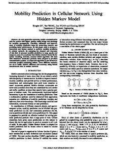
Figure 2. Prediction accuracy İ of eS(u) -Vote vs. the size s of the training set (in days) for different values of degree of randomness į.
TABLE I. Prediction Accuracy İ (%) vs. Degree of Randomness į for a 40-day training set.
IV. LOCATION PREDICTION EVALUATION
ǻ 0.00 0.25 0.50 0.75 1.00
We represent user trajectories through a series of waypoints. Each waypoint is defined by the location in terms of a cell and speed. The number of distinct cells is 100, hence, |Dom(em+1)| = 100. The synthetic traces were obtained by the RMPG tool [3] which allows controllable randomness. We have used five discrete levels of randomness from the regular pattern (į = 0, 500 training instances) to completely random trajectories (į = 1, 1000 training instances). We perform experiments with the Voting classification algorithm [8] which is implemented in the Weka ML workbench [2]. An important aspect of evaluation is how the prediction performance is affected by the size of the training set, s. Figure 2, shows the prediction accuracy of the eS(u)-Vote for training sets that correspond to 10, 20,…, 40 days. The window length m+1 is kept fixed at 4. The best performance is obtained for training sets of 40 days. We can observe that, as the size of the training set increases, so does the prediction accuracy. Better results are obtained for larger sets of the training data but complexity also raises (to a prohibitive level), hence we prefer to adopt limited size of training data (i.e., up to 40 days). The proposed model is evaluated with both synthetic data derived from RMPG [3] and realworld GSM cell-id data obtained from the MIT Media Lab Reality Mining project [5]. The realworld data refer to the movements of a MIT student during two and a half years (2004 to mid
İ of eS(u) - Vote 95.58 72.52 69.56 57.48 57.90
V. COMPARATIVE ASSESSMENT Previous work in the area of mobility prediction includes several models and approaches. We discuss the Kalman Filter (KF) based predictor [4] and the Hidden-Markov model approach for location prediction. We are mostly concerned with the complexity exhibited by these algorithms. The approximate pattern-matching algorithm – Hierarchical Location Prediction (HLP)- in [4] uses pre-recorded regular trajectories to estimate the inter-cell direction. Such algorithm uses an extended self-learning KF for unclassifiable random trajectories. HLP, which is a semi-Markov process, calculates l state transition probabilities. Each state refers to a discrete level of speed acceleration, thus, adding O(l2) space and time complexity. HLP uses the edit distance for matching an observation of dimension c⋅(m+1) (c is constant) to a pre-defined trajectory (of dimension m+1), thus, adding O(c⋅m2) time and O(m) space complexity. In our model, the distance calculation assumes only O(m) time and O(1) space complexity. Additionally, HLP highly depends on very specific spatial information that is, exact user position, speed, direction, cell geometry,
25 29
complexity O(m⋅s⋅log(s)) time complexity, the splitting of the two nodes in the 1st level assumes O(m⋅s⋅log(s/2)) time complexity, in the 2nd level O(m⋅s⋅log(s/4)), and so on. The classification time is proportional to the depth of the tree, i.e., O(log(s)) and the space complexity is proportional to the number of nodes, that is, O(s). Hence, the final classification complexity for our predictor ranges from O(1) + O(log(s)) to O(m⋅s) + O(log(s)).
cell residual time and overlapping areas among cells. Our predictor requires only the identifiers of the present and past cells visited by the user. HLP has to continuously track the user location, thus, leading to a large amount of historical data. In addition, due to such detailed information, HLP makes assumptions not well harmonized with mobile environments. HLP strictly depends on the underlying data as it assumes smooth movements. In our models, the adopted classifiers are trained for any distribution of the underlying information. Finally, HLP exhibits satisfactory prediction accuracy once the KF stabilizes: e reaches 0.72 for any į > 0.25. Our model can achieve this without the need for extensive historical information and data distribution assumptions. The adoption of a Hidden-Markov Model (HMM) as a possible predictor in our model (i.e., instead of k-nearest neighbor classifier and C4.5), presents the following drawbacks: (1) the time and space complexity [6], (2) the inability of HMM to classify totally unknown trajectories and, (3) the limited scalability of HMM when adding new, unvisited cells (all emission probabilities and probabilities of hidden states have to be recalculated). Specifically, by assuming the first e1 and last em cells of a vector e then the HMM calculates all possible hidden cell-transitions between e1 and em for the corresponding cells. This means that, HMM calculates the probability P(e) that the user produces a sequence e of m hidden cell-transitions. In our model with |Dom(e)| hidden states and a sequence of m+1 observations we obtain |Dom(e)|m+1 possible terms in calculating P(e), thus, leading to O(|Dom(e)|m(m)) complexity which is prohibitive. Note that the HMM forward algorithm reduces the computational complexity to O(|Dom(e)|2(m)) -far more efficient than the time complexity associated with exhaustive enumeration of paths- but stills leaves the space complexity unjustifiably high. The HMM adopted in [6] achieves performance comparable to our models at the expense of increased (location prediction) time complexity.
VI. CONCLUSIONS We proposed a location model for location prediction based on the user mobility behaviour. The model is evaluated through the 10-fold cross validation method with (i) sets of synthetic user movements with varying degrees of randomness and (ii) real-world location trajectories. We also report a computational analysis for our model. Our findings show that, the Voting classification scheme is appropriate for location prediction since it exhibits satisfactory prediction results for diverse user mobility behaviour and training set sizes. However, the model can be enhanced with more semantics and contextual information like temporal context (e.g., time period within a day), application context (e.g., service requests), proximity of people (e.g., social context) and destination and velocity of the user movement. Hence, the proposed location model representation should be able to support such data. Finally, the use of a combined model of several local models has to be considered in order to exploit local spatial and temporal information. REFERENCES [1] M. Plutowski, S. Sakata and H. White, Cross-validation estimates integrated mean squared error, Advances in Neural Information Processing Systems, vol. 6, 1994. [2] I. H. Witten and E.Frank, Data Mining: Practical Machine Learning Tool sand Techniques, Morgan Kaufmann Series in Data Management Systems, 2005. [3] M.Kyriakakos, N.Frangiadakis, S.Hadjiefthymiades and L.Merakos, RMPG: A Realistic Mobility Pattern Generator for the Performance Assessment of Mobility Functions, Simulation Modeling Practice And Theory, vol. 12, no. 1, Elsevier, 2004. [4] T. Liu, P. Bahl and I. Chlamtac, Mobility modeling, location tracking, and trajectory prediction in wireless ATM networks, IEEE JSAC vol. 16, no. 6, 1998. [5] http://reality.media.mit.edu/ [6] J-M Francois, G.Leduc, and S.Martin, Learning Movement Patterns in Mobile Networks: a generic method, proceedings of European Wireless, pp.128-134, 2004. [7] D. Lopresti, A. Tomkins, Block edit models for approximate string matching, Theoretical Computer Science, 181(1), 1997. [8] T. Anagnostopoulos, C. Anagnostopoulos, S. Hadjiefthymiades, M. Kyriakakos and A. Kalousis, Predicting the Location of Mobile Users: A Machine Learning Approach, ICPS 2009.
A. Computational Complexity
Our model uses s = |E| training vectors of (m+1)dimension for building the predictor. The complexity of k-nearest neighbor classifier corresponds to: O(m) for the distance calculation and O(m⋅s) for classification. However, a Voronoi tessellation implementation of k-nearest neighbor classifier exhibits complexity O(1) in time and O(s) in space by adopting the partial distance, search tree and editing algorithms [7]. Moreover, the adopted C4.5 (with binary splitting) results in O(s) + (s-1)⋅O(m) calculation time for splitting a training example. The total average time complexity for tree construction is O(m⋅s⋅(log(s))2) as long as the splitting of the root exhibits time
26 30