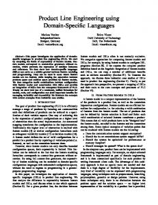
Model Checking of Domain Artifacts in Product Line Engineering. Kim Lauenroth, Klaus Pohl, Simon Töhning. Software Systems Engineering, ICB. University of ...
2009 IEEE/ACM International Conference on Automated Software Engineering
Model Checking of Domain Artifacts in Product Line Engineering Kim Lauenroth, Klaus Pohl, Simon Töhning Software Systems Engineering, ICB University of Duisburg-Essen 45127 Essen, Germany {kim.lauenroth| klaus.pohl|simon.toehning}@sse.uni-due.de several products of the product line and is thus costly to remove (cf. [19]; [22]; [26]). Model checking as a formal verification technique has received little attention in product line engineering so far. For verifying domain artifacts model checking approaches from single system engineering are only of limited use.
Abstract — In product line engineering individual products are derived from the domain artifacts of the product line. The reuse of the domain artifacts is constraint by the product line variability. Since domain artifacts are reused in several products, product line engineering benefits from the verification of domain artifacts. For verifying development artifacts, model checking is a well-established technique in single system development. However, existing model checking approaches do not incorporate the product line variability and are hence of limited use for verifying domain artifacts.
A. Model Checking of Domain Artifacts We define model checking of domain artifacts as follows: Model checking of domain artifacts means to verify that every possible product that can be derived from a domain artifact fulfills the specified properties. Thus, in contrast to model checking in single system development where a single product is verified if it fulfills the defined properties, model checking in product line engineering has to verify that a whole set of products fulfills the properties specified for each product. Several model checking approaches have been proposed for the verification of single system specifications (cf. e.g. [1]; [5]; [12]]) However, model checking approaches from single system engineering cannot directly be used for the verification of domain artifacts, since they do not consider the variability defined for the product line (cf. [18]). We will illustrate this using a simple example. Figure 1 depicts a simplified example for defining domain artifacts, properties and the variability of a product line. The example depicts a simplified orthogonal variability model, two I/O-automata and two properties (see Section II for a brief introduction into the modeling languages). The example specifies a simple product line for rail crossing gates which consists of a traffic light and a gate. The traffic light exhibits alternative variable behavior: The traffic light can either show a flashing yellow light or a steady yellow light when the gate is closing. The behavior can be verified with respect to the two variable properties. The variability is described by the variants of the variability model and by the relationships between the variants and the specification elements. If you ignore the variability model and apply a model checking approach from single system engineering to the example presented in Figure 1, the model checking approach would state that both defined properties are not fulfilled by the specified system, since it is possible to reach the states (yellow flash, closing) and (yellow, closing) which are counterexamples for the validity of each properties. However, this verification results is incorrect. The variability model does not allow to derive a product from the domain artifacts for which the property (closing + yellow) is
In this paper we present an extended model checking approach which takes the product line variability into account when verifying domain artifacts. Our approach is thus able to verify that every permissible product (specified with I/Oautomata) which can be derived from the product line fulfills the specified properties (specified with CTL). Moreover, we use two examples to validate the applicability of our approach and report on the preliminary validation results. Keywords: Product Line Engineering, Model Checking, Variability, Domain Artifact Verification
I.
INTRODUCTION
Model checking ([5]) is a technique for quality assurance that facilitates the verification of properties (typically specified in CTL) of a system (typically specified in a statetransition model). In software engineering for single systems, model checking is an established technique for verifying development artifacts in requirements engineering, design, realization, and test ([12]) in different domains such as in the automotive or avionic industry. Product Line Engineering is a development paradigm that explicitly addresses reuse by differentiating between two kinds of development processes (cf. [25], p. 21): In domain engineering, the domain artifacts of the product line are defined and developed. In application engineering, customer- and/or market-specific products are derived from the domain artifacts by binding the variability defined in the domain artifacts according to customer and/or marketspecific needs. The overall quality of the product line and its derived products mainly depends on the quality of the domain artifacts. In contrast to the development artifacts created in single systems engineering, the domain artifacts created in product line engineering are reused in several products derived from the product line. Thus, a high quality of the domain artifacts is desirable. A defect in a domain artifact typically affects
1527-1366/09 $29.00 © 2009 IEEE DOI 10.1109/ASE.2009.16
257 271 269
invariants, supports the model-checking of much richer property specifications. The remainder of this paper is structured as follows. In Section II, we present the modeling languages used to specify the domain artifacts in our model-checking approach. Our approach is presented in detail in Section III. A preliminary runtime evaluation of our approach is presented in Section IV and related work is discussed in Section V. A summary of our contribution and an outlook on future work is provided in Section VI.
specified and which is able to reach the state (yellow flash, closing), or vice versa for which the property (closing + yellow flash) is specified and which is able to reach the state (yellow, closing). orthogonal variability model VP
variation point
Close
V
V1: flashing yellow on closing
V
traffic light gate closed? gate closed? yellow flash
V2: yellow on closing
variants
II.
gate red
yellow
close gate? green close gate?
alternative variability dependency
open gate?
yellow red
gate open?
gate closed! close closing
close gate!
In this section, we introduce the languages used to specify the domain artifacts used in our model-checking approach.
open gate!
opening
open
SPECIFYING DOMAIN ARTIFACTS
A. Defining Product Line Variability For specifying the variability of a product line, we use the orthogonal variability modeling language developed in our research group ([25]). However, our model checking approach does not rely on the orthogonal variability model. Every other variability modeling language which can be formalized in the way presented in the following can be used instead such as, e.g., feature models (cf. [10]). The orthogonal variability model provides variation points, variants, variability dependencies, and constraint dependencies to define the variability of a product line. Variation points are differentiated into mandatory variation points which have to be considered and optional variation points which might be considered if required. Variability dependencies define the allowed selection of a variant at a variation point. We differentiate between mandatory (must be selected), optional (can be selected), and alternative (selection out of a defined set of variants). Constraint dependencies define constraints for the selection of variants and variation points. We distinguish between requires dependencies and exclude dependencies. A simplified example of a variability model is depicted in the upper part of Figure 1. Details about the definition of our variability model and on the documentation of product variability can be found in [24] and [25]. Formally, the variability model is interpreted as a set of variants V where each variant vi is represented by a Boolean variable. We represent a selection of variants of the variability model as a vector v = (v1, …, vn) over the variants: � vi is set to true if the variant vi is selected
gate open!
properties If gate is closing, light is flashing yellow (closing Ö yellow flash). If gate is closing, light is yellow (closing Ö yellow).
Figure 1. Simplified Example of Domain Artifacts
A way to apply model checking approaches from single system engineering in product line engineering would thus be to derive every possible product from the domain artifacts and then verify each derived product individually. Since thousand or even more products can be derived from a product line (cf. [25], p. 418), this is impractical in most cases. B. Goal and Contibution of this Paper This paper aims in extending existing model checking approaches to facilitate the verification of domain artifacts in product line engineering. The contribution of this paper is threefold: 1) We investigate in model checking problems faced in product line engineering mainly caused by the variability of the domain artifacts. 2) We present a model checking approach for verifying domain artifacts in product line engineering which takes the variability defined for the product line into account. 3) We demonstrate the applicability of our approach by applying our tool prototype to an extended example. The approach presented in this paper is a significant improvement of our previous work on consistency checking of domain artifacts in product line engineering (cf. [18]; [19]). In [19], we examined the consistency problem of domain artifacts and defined a general framework for consistency checks of domain artifacts. In [18], we presented an approach based on this framework for model-checking based consistency checks between automata and invariants in product line engineering. In contrast, the approach presented in this paper supports model-checking of properties specified in CTL and thus, compared with our previous work which just focused on
�
vi is set to false otherwise
Variation points are also formalized as Boolean variables. The value of a variation point variable is determined by the kind of variation point. The variable of a mandatory variation point is always set to true, whereas the variable of an optional variation point can be set to true or false. The value of an optional variation point is determined by the constraint dependencies of the variability model. The variability and constraints dependencies of the variability model are translated into Boolean expressions over the variables of the variation points and variants. Let VD = {vd1, …, vda} be the set variability dependencies, and 270 272 258
�
let CD = {cd1, …, cdb} be the set of constraint dependencies. The variability model is captured by the function OVM over the variants V: OVM(v) = Rvd � VD vd Z R cd � CD cd. The function OVM(v) evaluates to true, if the selection of variants satisfies all variability dependencies and all constraint dependencies, and otherwise to false. For more details on the formal specification of the orthogonal variability model, we refer to [24]. As argued in [19], verifying domain artifacts requires to check whether the variability model allows the selection (or de-selection) of a set of variants. For example, we might want to check if the variants v1 and v2 can be selected together when, at the same time, v3 is not selected. We therefore define the function SAT-VM as follows. The function has two inputs: the function OVM as introduced above and a Boolean expression V* over the variants of the variability model to represent the desired selection (e.g. v1 Z v2 Z \v3 for the given example). SAT-VM(OVM, V*) evaluates to true, if V* can be fulfilled in the given function OVM, and to false, if not. The calculation of the function SAT-VM is NP-complete, since it is a special case of the Boolean satisfiability problem (SAT) which is known to be NP-complete. The worst case runtime of SAT-VM is therefore exponential. However, current SAT solver algorithms are able to handle variability models in an acceptable time (cf. [[8]; [18]; [24]). We therefore neglect the runtime of the function SAT-VM.
May transitions can be selected to become part of a derived automata specification
An I/O-automaton can be derived from a modal I/Oautomaton by selecting a set of may transitions from the defined may transitions and by transferring all must transition into the derived I/O-automaton. However, Larsen et al. did not include the possibility to specify constraints between may transitions (e.g., the selection of one transition requires the selection of an additional transition). Such constraints are typically specified in product line engineering using a variability model. In the following, we combine our orthogonal variability model presented in Section II.A with I/O-automata to enable the specification of such constraints. Instead of our orthogonal variability model, it also possible to use feature models or decision tables for this purpose. We have chosen the orthogonal variability model because of our positive experience with our industrial partners. The orthogonal variability model provides the concept of artifact dependencies between variants and specification elements in order to specify that a specification element is variable (cf. [25]). For example, in Figure 1 the transition is related to the variant V1 by an artifact dependency (dashed line). This relation expresses that this transition is only part of a derived specification, if the variant V1 is selected. The transition is related to the variant V2. The variability model defines the variants V1 and V2 as alternative, i.e., both variants cannot be selected together. Thereby, both transitions can never become part of a derived specification. The modal I/O-automata presented by Larsen et al. are not capable of specifying such information. Therefore, we combine modal I/O-automata and the orthogonal variability model to define a variable I/Oautomata specification as follows. A variable I/O-automaton specification consists of an orthogonal variability model with a set of variants V as defined in Section II.A, a set of variable I/O-automata C = {C1, …, Cx}, and a variability relation VRelIO. A variable I/O-automaton Ci is defined as 6-tuple (Zi, z0,i, Sendi, Receivei, Ti) where � Zi is the set of states � z0,i � Zi is the initial state � Sendi is the set of sendable messages (a sendable message is followed by a ‘!’) � Receivei is the set of receivable messages (a receivable message is followed by a ‘?’) � Ti Zi u M u Zi (M = Sendi Receivei) is the transition relation.
B. Variable I/O-Automata For the specification of the system, we use I/O-automata which are an established language for modeling concurrent and distributed discrete event systems ([23]) and are also used for specifying domain artifacts ([17]). Similar to the orthogonal variability model, our approach does not rely on I/O-automata. One could use any other language which could be transformed into a global system automaton. In Section D, we illustrate the product construction of variable I/Oautomata in order to create a variable global system automaton. In I/O-automata specifications, the specified system is separated into different components where each component is modeled by a state automaton. The different components communicate with each other via message exchange. This is realized by transitions which either can send a message (indicated by an ‘!’) or receive a message (indicated by an ‘?’). Furthermore, I/O-automata can perform internal actions that do not influence other automata. Without loss of generality, we assume deterministic behavior, since every non-deterministic automaton can be transformed into a deterministic one. The lower part of Figure 1 shows a simple example of an I/O-automaton. With respect to product line engineering and I/Oautomata, Larsen et al introduced the concept of modal I/Oautomata to specify a set of I/O-automata within a single model automaton (cf. [17]). Modal I/O-automata separate two kinds of transitions: � Must transitions are part of every derived automata specification
The variability relation VRelIO V u (Ti) documents the artifact dependency ( denotes the power set) between the variants of the orthogonal variability model and the transitions of the I/O-automata in order to define which transitions are common and which are variable: � A transition t � Ti is variable (i.e. a may transition as defined by Larsen et al.), if t is related to a variant, i.e. M(v, T’) � VRelIO: t � T’
271 273 259
�
�
A transition t � Ti is common (i.e. a must transition as defined by Larsen et al.), if t is not related to a variant, i.e. L(v, T’) � VRelIO: t � T’
A CTL property p’ � CTL is common, if t is not related to a variant, i.e. L(v, P) � VRelCTL: p’ � P.
Again, we assume that a property cannot be related to more than one variant (see Section II.B), i.e. �(v1, P1), (v2, P2) VRelCTL: (P1 P2 = ) (v1 = v2). The derivation of the CTL properties of a particular system takes place in the same way as the derivation of a variable I/O-automaton (see Section II.B).
Without loss of generality, we assume that a transition cannot be related to more than one variant, i.e. �(v1, T’1), (v2, T’2) VRelIO: (T’1 T’2 = ) (v1 = v2), since every orthogonal variability model with multiple artifact dependencies between variants and artifacts can be transformed into an orthogonal variability model with a unique artifact dependency. A proof of this claim can be found in [20]. The derivation of an I/O-automaton from a variable I/Oautomaton takes places as follows. Let Ɩ = (v1, ..., v|V|) (true, false)|V| with OVM(Ɩ) = true be a selection of variants that satisfies the variability model. The set T of transitions of the derived I/O-automaton is defined as follows: T = {t Ti | �(vi, T’’) VRelIO: t T’’ vi = true} {t Ti | N(v, T’’) VRelIO: t T’’}
D. Product Construction of Variable I/O-Automata In order to facilitate the model checking of variable I/Oautomata specifications as introduced in Section II.B, a product construction has to be performed to merge the different I/O automata into a single automaton. In [18], we have shown that variability has to be included into the product construction process for variable deterministic automata. However, our approach presented in [18] does not include sending and receiving transitions specified in I/Oautomata. In the following, we present an extension of our approach that includes sending and receiving transitions.
C. Variable Computational Tree Logic For the documentation of the system’s properties, we use the Computational Tree Logic (CTL, cf. [5]). CTL is an extension of classical logic amongst a time dimension in order to specify behavioral properties of a system which are used to verify a system specification (cf. [5]). The CTL contains quantifiers over paths and pathspecific quantifiers. Clarke et al. have shown that Y, \, EG, EU, and EX represent a minimal set of CTL operators, i.e. that every CTL expression can be transformed into a CTL expression that consists of these operators (cf. [6]). The operators have the following meaning: � f1 Y f2, is the logical OR and evaluates to true, if f1 or f2 is true � \f1 is the logical NOT and evaluates to true, if f1 is false � EG f1 evaluates to true, if there is one path starting at the initial state on which f1 is always true � E [f1 U f2] evaluates to true, if there is one path starting at the initial state on which f1 holds at least for one state and in the next state f2 holds. � EX f1 evaluates to true, if there is one path starting at the initial state on which f1 holds on the next state.
z1-1
a! (v1)
component 1
z1-2
z2-1
a? (v2)
z2-2
component 2
Figure 2. Excerpt of a variable I/O-automata specification
Figure 2 depicts an excerpt of a variable I/O-automata specification with two components. The related variants of the transitions are documented within parentheses. Assume that the specified system is in the state (z1-1, z2-1). With respect to the selection of variants, the following cases are possible: � v1 and v2 are selected: both transitions are present in the system, i.e. component 1 can send message a and component 2 can receive message a. The system changes to the state (z1-2, z2-2). � v1 is selected: only the transition in component 1 is present, i.e. component 1 can send message a, but component 2 cannot receive message a. The system changes to the state (z1-2, z2-1). � v2 is selected: only the transition in component 2 is present, i.e. component 2 can receive message a, but component 1 cannot send message a. The system cannot change its state. � v1 and v2 are not selected: both transitions are not present in the system, i.e. the system cannot change its state.
In order to define CTL properties for I/O-automata, we adapt the approach from Behrmann et al. [2] who assume that the names of the states are used as Boolean properties. For example, if the system described in Figure 1 is in the states red and closed, the properties red and closed are fulfilled (i.e. true). All other properties (e.g., green, closed, etc.) are not fulfilled (i.e. false). In order to enable variability for the CTL properties, we define a variability relation VRelCTL´ V u (CTL) for a set of CTL properties specified in the set CTL: � A CTL property p’ � CTL is variable, if p is related to a variant, i.e. M(v, P) � VRelCTL: p’ � P. The property p has to be fulfilled only if the related variant v is selected.
This example shows that the presence and absence of variable transitions has to be included into the product construction. In order to realize this, we define an extended transition relation which includes the variability information (i.e. selection or deselection of variants). Let Ki = (Zi, z0,i, Sendi, Receivei, Ti) be a variable I/O-automaton and VRelIO be the variability relation introduced in Section II.B, and let V* be the set of positive and negative variants. The extended
272 274 260
transition relation Ti* Zi u (Sendi Receivei) u Zi u (V*) is defined as follows: Ti* = (1) {z1mz2V’ | �z1mz2 Ti �V’ (V*): V’ = { v | �(v, T’) VRelIO: z1mz2 T’} { v | �z1mz’ Ti �(v, T’) VRelIO: z1mz’ T’}} (2) {z1mz2 | �z1mz2 Ti �(v, T’) VRelIO: z1mz2 T’ } (3) {z1mz2V’ | �z1mz2 Ti m Receivei �(v, T’) VRelIO: z1mz2 T’ �V’ (V*): V’ = {v | �z1mz2 Ti �(v, T’) VRelIO: z1mz2 T’} The extend transition relation captures three kinds of transitions: 1) Variable transitions: For variable transitions, T* captures the related variant and the variants that must not be selected in order to ensure deterministic behavior. 2) Common transitions: Common transitions (i.e. transitions that are not related to a variant) become part of T*. The set V’ remains empty, since a common transition is not related to a variant. 3) Implicit transitions: For states with receiving variable transitions, additional transitions are added to T* which capture the behavior in the case that the related variant is not selected. Based on the extended transition relation, we define the product of two variable I/O-automata as follows: � The set of states is the product of both state sets: Z12 = Z1 u Z2 � The start state is the combined start state of both automata: z012 = z0,1z0,2 � The set of sendable messages is the union of both automata: Send12 = Send1 Send2 � The set of receivable messages is calculated as follows Receive12 = (Receive1 \ Send2) (Receive2 \ Send1)
�
Case 3: The second components automaton sends or receives a message that cannot be processed by the first components automaton. This case is analog to the second case. {z1z2mz1z2’V2’ | N z1mz1’V1’ T1* � z2mz2’V2’ T2* (m Send2 m Receive12)}}
The product construction is defined for two automata. The product construction of more than two automata is performed in pairs. III.
MODEL CHECKING VARIABLE I/O-AUTOMATA
In this section, we present our approach for the model checking of variable I/O automata. Our approach is based on the model checking approach from Clarke et al. (cf. [5]) which is considered as one of the fundamental approaches for model checking. The central idea of our approach is to include the variability information specified in the variability model (as Boolean variables) into the model checking algorithms. During the exploration of the state space, the algorithms consider the variability model to ensure that the current path explored in the state space is valid with respect to the variability model. Our adaptation is threefold: 1) Adaptation of state labeling: The approach from Clarke et al. (cf. [5]) labels each state with the properties that are fulfilled in this state. In variable I/O-automata, the fulfillment of a property may rely on variable transitions. Therefore, the state labeling may include the variant selection which is necessary to fulfill the property. We elaborate on this extension in Section III.A. 2) Adaptation of algorithms: We adapt the algorithms for model checking of EX, EU, and EG. This is sufficient since all other expression can be reduced to a combination of the EX, EU and EG operators [6]. The adaptations are presented in the Sections III.B to III.D. It is not necessary to adapt the procedures for handling expressions of the form \f1 and f1 Y f2 because the results of the computations only depend on single states. 3) Checking the completeness of witnesses: The existing single system algorithms rely on witnesses to show that a property is fulfilled for a given system (cf. [6]). This approach is not sufficient for variable I/O-automata, since a variable I/O-automaton represents a set of systems and thus a witness must exist for every possible system. In Section III.E, we address this problem by checking the completeness of witnesses for all possible systems. All presented algorithms assume that the variable I/Oautomaton with the start state z0 and the extended transition relation T* are available as global variables (see Section II.D) and the variability model is accessible by the function SAT-VM (see Section II.A).
The combined transition relation T12* has to distinguish three cases in order to include the variability: � Case 1: The transitions of both components’ automata fits each other (i.e. one component sends a message that can be received by the other or both components receive the same message), and the variants of both transitions fit each other (i.e. the variants do not contradict each other). {z1z2mz1’z2’(V1’ V2’) | �z1mz1’V1’ T1* �z2mz2’V2’ T2* (V1’ V2’ false)} � Case 2: The first components automaton sends or receives a message that cannot be processed by the second components automaton. In this case, the first components automaton executes the transition and the second component remains in its current state. {z1z2mz1’z2V1’ | �z1mz1’V1’ T1* N z2mz2’V2’ T2* (m Send1 m Receive12)}
273 275 261
Each presented adaptation consists of three parts. First, we discuss the need for the adaptation. Secondly, we describe the adaptation itself. Finally, we present a brief argumentation for the correctness of the adaptation and briefly discuss the runtime of the presented adaptation.
(5) (6) } } }
The algorithm works as follows. For each outgoing transition of each state of a variable I/O-automaton, the algorithm checks the following. If the reached state z2 is labeled with f1 and the combined selection of variants of the property (i.e. vEX), the current transition (i.e. V’), and the selection of variants associated with f1 in the next state (i.e. VP) can be fulfilled, then the state z1 is labeled with (EX f1, (vEX Z V’ Z VP)) (line (5) and (6)). This label documents that EX f1 is fulfilled, if the variants documented by (vEX Z V’ Z VP) are selected. If the start state z0 is labeled, a witness for EX f1 has been identified. In Section III.E, we will check the completeness of witnesses with respect to all possible products of the considered product line.
A. Adaption of State Labeling 1) Need for Adaption: Figure 3 shows an example of a simple variable I/Oautomaton with two states. The state z1 is labeled with the property f1. Since state z0 has a transition to the state z1, the state z0 can be labeled with EX f1. However, the transition between both states is related to the variant v1, i.e. the transition is only present, if v1 is selected. Therefore, the fulfillment of the property EX f1 relies on the selection of v1, since the property is not fulfilled, if the transition is not present. Consequently, the fulfillment of a property may rely on the selection of variants. (EX f1, v1)
x (v1)
z0
label(z1) = label(z1) F (EX f1 ; (vEX Z V’ Z VP))
3) Correctness and Runtime The correctness of the presented adaption follows from the following observation. The algorithm checks each outgoing transition of each state and all possible labels. Therefore, every possible witness for EX f1 will be identified. The worst case runtime of the presented algorithm is linear in the number of transitions and labels, since every transition is considered only once by the algorithm. For each transition, the algorithm considers each labels of the destination state of the considered transition.
f1 z1
Figure 3. Example of the influence of variability on a property
2) Adaption of Algorithm To incorporate the variability, we extend the labeling procedures introduced by Clarke et al. (cf. [5]) as follows. Let f1 be an expression, let z � Z be a state of an I/Oautomaton, and let V’ be a (possibly empty) selection of variants. The state z is labeled with (f1, V’) (i.e. (f1, V’) � label(z)), if f1 is fulfilled in state z for the selection V’ of variants.
C.
Adaptation of Model Checking E[f1 U f2]
3) Rutime of Adaption The presented adaptation does not change the runtime of the labeling procedure, since our adaptation only adds information to the state labeling. B. Adaptation of Model Checking EX f1
1) Need for Adaption To handle expressions in the form E[f1 U f2], it is first necessary to find every state which is labeled with f2. Then, a backward search is performed from these states to find a path to the start state whose states are labeled with f1. Similar to EX f1, it is necessary to include the variability of the transitions and the properties in order to determine whether a witness exists or not.
1) Need for Adaption For the property EX f1, basically every state should be labeled with EX f1 which has some successor state that is labeled with f1. Since the transitions in a variable I/Oautomaton and the property f1 can be variable, it is necessary to check whether the variants related to f1, to the considered transition, and to EX f1 can be selected together.
2) Adaptation of Algorithm Algorithm 2 shows the adaption of this procedure to handle model checking of E[f1 U f2] in a variable I/Oautomaton. The algorithm has three parameters: The properties f1 and f2, and the variant vEU which is related to E[f1 U f2]. The variant vEU is empty, if E[f1 U f2] is a common property.
2) Adaption of Algorithm Algorithm 1 shows the calculation of the expression EX f1 for a variable I/O-automaton. The algorithm has two parameters: First the property f1 which should be checked and secondly the variant vEX which is related to EX f1. The variant vEX is empty, if f1 is a common property.
Algorithm 2: Checking E[f1 U f2] (1) CheckEU(f1, f2, vEU){ (2) Z’ := { (z, vz) | (f2 ,vz) � label(z) Z SAT-VM(OVM, vZ Z vEU)} (3) for each (z, vz) � Z’ { (4) for each z’nz V’ � T*, with z’ z { (5) if(SAT-VM(OVM, (vZ Z vEU Z V’ ))) (6) PathSearch_EU(f1, z', t, (vZ Z vEU Z V’ )); (7) } } }
Algorithm 1: Checking EX f1 (1) checkEX(f1, vEX){ (2) for each t = z1nz2 V’ � T* { (3) for each (f1, VP) � label(z2) (4) if(SAT-VM(OVM, vEX Z V’ Z VP))
(8) PathSearch_EU(f1, z, path p, Variants V* ){ (9) if ((f1, vP) � label(z) Z SAT-VM(OVM, (vP Z V*)) {
274 276 262
D.
(10) label(z) = label(z) F (E [f1 U f2], (vP Z V*)); (11) if(z != z0) { (12) for each z’nz V’ � T*, with z’ � p { (13) if(SAT-VM(OVM, (V’ Z vP Z V*)) (14) PathSearch_EU(f1, z', t F p , (V’ Z vP Z V*)); (15) } } } }
Adaptation of Model Checking EG f1
1) Need for Adaption As mentioned above, EG f1 evaluates to true if there is a path from the start state on which f1 is always true. The computation in the non-variable case is based on the restriction of the automaton to states which fulfill f1 and a decomposition of this restricted state graph into nontrivial strongly connected components (SCC) [6]. This step is performed by using the algorithm of Tarjan [27] for detecting SCC. Then, a backward search is performed to find any state in the restricted automaton that can reach an SCC. If the start state is reached, a witness for EG f1 is found. However for model checking of EG f1 in a variable I/Oautomaton it is not sufficient to search for states that reach an SCC. The following problems occur if we proceeded in this manner: � An SCC could be not valid regarding the variability model, see Problem (a) in Figure 4: variant v2 excludes variant v3 and therefore both variants cannot be selected together, i.e. that the identified SSC will never become part of a derived product. � Searching for an identified SCC could fail although a valid witness for EG f1 exists; see Problem (b) in Figure 4. The identified SCC covers the variants v1 and v3. The backward search checks the transition related to v2 and fails since v2 and v3 cannot be selected together. However, there is a witness without v3, since a path and an SCC exists on which f1 is always true in the product which contains v1 and v2. � Searching for states that reach an SCC could result in an incomplete set of witnesses, see Problem (c). The backward search labels state z0 with EG f1 which reaches an SCC (V* = v1 Z v3). Therefore, the witness is valid for a product which contains the variants v1 and v3. State z0 reaches yet another path for a product which only contains variant v1 on which f1 is always true, but this is not considered.
The algorithm works as follows. First, it determines the states z that are labeled with f2 for which the orthogonal variability model can fulfill the variant selection (vZ Z vEU), i.e. it is possible to derive a product which contains a state that is labeled with f2 (line (2)). For each incoming transition of such a state z, the algorithm checks whether the orthogonal variability model fulfills the variant selection (vZ Z vEU Z V’), i.e. whether the considered transition is also part of the derived product which contains the state labeled with f2 (line (3) – (5). If the orthogonal variability model can fulfill this selection, the backward search is started in a recursive manner (see line (6)) to determine further states that fulfill f1. The algorithm for the backward search has parameters for the property f1, the current state z of the backward search, the path p to the current state and the selection of variants V* that must be selected in order to visit the transitions of the path p. For the initial call of the function, V* contains the variant vEU which is related to E[f1 U f2], the variant vz related to f2, and the variant selection V’ which is related to the variable transition. The first step is to check if state z is labeled with f1 and if the variant selection related to f1 can be fulfilled by the orthogonal variability model together with V* (line (9)). If yes, the state is labeled with (E [f1 U f2], (vP Z V*)) (see line (10)). If the current state is the start state z0, a witness for E [f1 U f2] has been identified. In Section III.E, we will check the completeness of witnesses with respect to all possible products of the considered product line. If the current state is not the start state, the next step of recursion is performed for each incoming transition if the variant selection V’ of the transition, the variant vp, and the variant selection V* can be fulfilled by the variability model (line (13) and (14)). The algorithm avoids entering a state twice in order to avoid circles in the considered path (see line (4) and line (12)). 3) Correctness and Runtime The correctness of the presented adaption follows from the following observation. The algorithm checks every possible state that is labeled with f2. Therefore, no possible initial state for E[f1 U f2] is missed. For every possible initial state, a comprehensive path search is performed, therefore no possible witness for E[f1 U f2] is missed. The path search is comprehensive, since the path search performs a complete depth first search of the automaton. The worst case runtime of the presented algorithm is exponential in the number of states, since, in the worst case, the path search has to check every possible path through the automaton. And, the number of possible paths in an automaton is exponential in the number of states.
Figure 4. Problems of model checking EG f1 in variable I/O-automata1
1
275 277 263
The transitions in this figure are only labeled with variants.
In summary, an SCC which was found by Tarjans algorithm does not have to be a valid SCC in a variable I/Oautomaton (see Problem (a)). Searching for an SCC in a variable I/O-automaton depends on the state at which the search is started (see Problem (b)). Additionally, it is not sufficient to consider only the maximal SCC, because an SCC could contain several paths, which are witnesses for different products (see Problem (c)).
(22) } } (23) z.visited:= false; (24)} }
If no cycle is detected, the next step of the recursion is further performed for each outgoing transition if the variant vP, the variant selection V’, and the selection of Variants V* fulfill the variability model and the successor is labeled with f1, see line (20). Before this step the current state is labeled as visited, see line (18).
2) Adaptation of Algorithm Algorithm 3 considers the problems mentioned above. The central idea is to consider only single cycles within the automaton whereas an SCC identified by the algorithm of Tarjan may contain several cycles which leads to the problems mentioned above. The algorithm has two parameters: First the property f1 which should be checked and secondly the variant vEG which is related to EG f1. The variant vEG is empty, if EG f1 is a common property. The algorithm works as follows. For each outgoing transition, for each state which is labeled with f1, a depth first search for a cycle which fulfills the variability model is started recursively by calling the method FindPathToCycle, see line (8). Before this, the current state is marked as visited, see line (4). FindPathToCycle is only called if the variant selection V’, which is related to the transition to the successor can be fulfilled together with the variant vp and if the successor is labeled with f1. The method FindPathToCycle has parameters for state zinitial from which the search is started, state z for the successor state, and the selection of variants V* that must be selected in order to visit the transitions of an already visited path. In line (13), the algorithm checks whether the current state has been visited. If yes, a cycle is found that fulfills the variability model and on which every state is labeled with f1. The state zinitial is labeled with EG f1 and the selection of variants V*.
Figure 5. Exemplary result for EG f1 1
Because we start a new depth first search from each state which is labeled with f1, the algorithm resets the visited flag for each state after a complete execution of recursion, see line (10) and (23). The result after a complete execution of Algorithm 3 is as follows. Every state which is labeled with f1 and which reaches a cycle in the variable I/O-Automaton or is part of such a cycle is labeled with EG f1 and with a selection of variants for which the labeling is valid, see Figure 5 for an example. The start state z0 is labeled with EG f1 for products that consist of variants v1 and v2 or variant v1 or variant v1 and v3. Therefore, we have a witness for EG f1 for each possible product of the product line, see the orthogonal variability model in Figure 5.
Algorithm 3: Checking EG f1 (1) CheckEG(f1, vEG){ (2) Z’ := { (z, vz) | (f1, vz) � label(z) Z SAT-VM(OVM, vZ Z vEG)} (3) for each z � Z’ { (4) z.visited :=true; (5) for each znz’ V’ � T* { (6) if(SAT-VM(OVM, V’ Z vEG Z vz)) { (7) if(f1 � label(z’)) { (8) FindPathToCycle(z, z‘, t, V’ Z vEG Z vz); (9) } } } (10) z.visited:=false; (11)} }
3) Correctness and Runtime The correctness of the presented adaption follows from the following observation. The checking algorithm identifies every possible state that is labeled with f1 and starts a comprehensive path search for cycles from each state. Therefore, no possible witness for EG f1 can be missed. The path search is comprehensive, since it uses the depth first search approach. The worst case runtime of the presented algorithm is also exponential in the number of states, since, in the worst case, the path search has to check every possible path through the automaton. And, the number of possible paths in an automaton is exponential in the number of states.
(12)FindPathToCycle(zinitial, z, V*) { (13) if (z.visited) { (14)
E.
label (zinitial) := label(zinitial) � (EG f1, V*);
1) Need for Adaptation As argued above, finding one witness for EX, E[f1 U f2] and EG f1 is not sufficient for ensuring that every I/Oautomaton that can be derived from the variable I/Oautomaton fulfills its CTL properties. One witness is a
(17) } else { (18) z.visited:=true; (19) (20) (21)
Checking Completeness of Witnesses
for each znz’ V’ � T* { if ((f1, vP) � label(z’) Z SAT-VM(OVM, (vP Z V’ Z V*)) { FindPathToCycle(z0, z‘, (vP Z V’ Z V*));
276 278 264
The selection (\v1 Z \v2) can be fulfilled by the orthogonal variability model presented in Figure 6, since it is possible to select only the variant v3 what we have already identified above.
witness for one or more products; and we have to check if it is possible to derive a product which contains no witness for its CTL property. We illustrate this using a simple example in Figure 6. f1
VP
vp 1
f1 v1
V
v1
V
v2
V
v3
3) Correctness and Runtime The correctness of the presented algorithm follows directly from line (2), since line (2) realizes the query described in Section III.E.2). The runtime of algorithm 4 is linear in the number labels related to the property f that are defined for the state z, since the construction of the Boolean equation in line (2) has to consider every label defined for state z, whether it is related to f or nor.
\f1 v2
v3
(EX f1, v1) z0 (EX f1, v2)
Figure 6. Example of checking the completeness of witnesses
Figure 6 shows an example for the result of model checking EX f1 where we assume that EX f1 is a common property, i.e. it has to be fulfilled by every possible product. The initial state z0 is labeled with two labels for EX f1, one for the variant v1 and one for the variant v2, i.e. there are witnesses for EX f1. However, this set of witnesses is not complete. The orthogonal variability model on the left hand side in Figure 6 defines the three variants v1 to v3 as alternative, i.e. exactly one of the three variants has to be selected. Therefore, it is possible to derive a product which only contains the variant v3 and for this product, there is no witness for EX f1 since it is impossible to reach a state from z0 that is labeled with f1. A similar example can be defined for the other two properties.
IV.
EXAMPLE AND RUNTIME EVALUATION
The runtime estimation of our presented approach indicates an exponential worst case runtime for the verification of EU and EG properties. In order to determine the runtime behavior of our approach, we have realized the approach in a prototypical tool environment in order to apply it to examples. We applied our approach to two examples and verified for each example one property of each type (i.e. EX, EU, and EG). The first example is a small sample specification. It consists of five variable I/O-automata and an orthogonal variability model which specifies six variation points and 14 variants. Overall 189 products can be derived from this specification. The product automaton of the specification consists of 12.000 states and 29.000 transitions. The second example is a (realistic) specification consists of six variable I/O-automata and the orthogonal variability model of the specification consists of ten variation points and 46 variants and allows the derivation of 237 different products. The product automaton of the specification consists of more than 68.000 states and 174.000 transitions. For the execution of our approach, we used a standard desktop PC with an Intel Core 2 Duo 6400 CPU with 2.13 GHz and 2 Gb RAM. The following table depicts for each property (EX, EU, EG) the runtime consumed for the product construction (see Section II.D) and the runtime consumed for verifying the individual properties (see Section III).
2) Additional Algorithm Since approaches from model checking for single systems do not need to check the completeness of witnesses, we have to define an additional algorithm. Algorithm 4 presents the completeness check for witnesses. The algorithm has three parameters: the property f and the state z for which the completeness check has to be performed, and the variant v which is related to the property f. The variant v is empty, if f is a common property. Algorithm 4: Checking Completeness of Witnesses (1) checkCompletness(f, z, vp){ (2) if(SAT-VM(OVM, vp Z (R(f, V’) � Label(z) \V’) = false) (3) output “There is a witness for each product”; (4) else (5) output “There is at least one product without a witness”; (6) } }
Runtime (sample specification)
The algorithm works as follows. It checks in line (2) if the orthogonal variability model can fulfill a variant selection in which vp is selected and all possible variant selections related to the witnesses for f are not selected (i.e. (R(f, V’) � Label(z) \V’)). If this is not possible, it is not possible to derive a product which has no witness for the property f in state z. If such a variant selection exists, this variant selection is an example for a derived product that has no witness for the property f. For the example given in Figure 6, the check would be performed as follows. Line (2) would check the following formula (vp is empty, since EX f1 is common what we represent by the Boolean value true):
Runtime (realistic specification)
Property 12.000 states / 29.000 transitions 68.000 states / 174.000 transitions ProductProductVerification Verification construction construction EX 99,72sec 0,27sec 203,7sec 1,7sec EU 100,08sec 0,25sec 202,8sec 0,75sec EG 99,92sec 4,25sec 202,7sec 32,93sec
From this initial runtime evaluation we conclude that: 1) In both examples, the product construction requires a large amount computation time. This is not surprising, since the product construction suffers from the so called state explosion problem (cf. [6]), i.e. the runtime of the product construction grows exponentially with the number of component automata.
SAT-VM(OVM, (true Z (\v1 Z \v2))
277 279 265
C. Model Checking of Partial State Spaces Brunns and Godefroid (cf. [4]) present a model checking algorithm for partial state spaces with uncertain states. Their algorithm performs pessimistic and optimistic searches. A pessimistic search assumes that all uncertain states are absent whereas an optimistic search assumes that all uncertain states are present. This approach is not applicable to the variability of domain artifacts, since the fulfillment of properties must be verified for each permissible combination of variants, not only for special cases such as “all variants absent” or “all variants selected”. The variability model might even exclude these cases (e.g. by defining the variants of a variation point as mutually exclusive).
2) For both examples, the verification of an EX property is fast compared with the overall runtime (0,27% for the first and 0,83% for the second example). This supports the results of the runtime evaluation (cf. Section III.B.3) which showed that the verification of EX requires linear runtime. 3) In both examples, the verification of an EU property is fast compared with the overall runtime for both examples (0,25% in the first and 0,37% in the second example). This result is surprising since the runtime evaluation in Section III.C.3) indicates an exponential runtime in the worst case 4) For both examples, the verification of an EG property requires significantly more time (4% in the first and 14% in the second example) compared with the runtime required for verifying the other two properties (EX and EU). This supports the results of the runtime evaluation in Section III.D.3) which indicates that the verification of EG required exponential time. V.
D. Model Checking and Verification of Domain Artifacts Classen et al. [7] describe the general problem of determining whether a set of features can be composed as a problem called “safe composition”. Several researchers address this problem. Batory and Thaker [28] support the automatic creation of a product line software implementation based on feature models. They focus on the safe composition of products by ensuring that there is no undefined element (e.g. classes, method) referred to in a composed program implementation. Batory and Thaker deal with static properties of the product line and do not support a consistency check of behavioural properties. In [9] Delaware et al. extend this approach by introducing Lightweight Feature Java (LFJ), a language to formalize feature-based product lines. Additionally they define a constraint based type system for LFJ. If any composition of features satisfies the typing constraints all programs allowed by the feature model are type safe. However, like in [28], they only proof type safety at source code level. Czarnecki and Pietroszek [8] propose an approach to verify feature-based model templates against OCL-based well-formedness rules. They check whether an instance of the model template exists that violates the predefined wellformedness rules. Their approach can be applied to a domain artifact. However, Czarnecki and Pietroszek only deal with static properties of the UML and do not consider dynamic properties. Gruler et al. [13] extend the process algebra CCS and the ȝ-calculus in order to support the formal specification and verification of product lines. However, variability constraints are not supported by the approach. Furthermore, the automated verification using a verification tool is not considered, which is prerequisite for a practical evaluation. Kästner and Apel [14] extend the Featherweight Java calculus with annotations to be used for Software Product Lines. With this extended calculus they can prove, if the Software Product Line is well typed, that all possible variants are well typed. In contrast to our approach they only perform a static analysis of source code fragments. Kishi et al. [16] propose an approach which supports the formal verification of a product specification derived from the domain requirements specification in application engineering. In [15], Kishi and Noda briefly sketch a technique that is applicable in domain engineering. This technique derives a set of potential products and verifies
RELATED WORK
A. Symbolic Model Checking The concept of Boolean expressions related to transitions in symbolic model checkers such as NuSMV [3] is similar to the concept of variants which are related to transitions to indicate variability. This makes it possible to use guards to encode the model checking problem presented in this paper and thereby apply existing symbolic model checking approaches. However, this solution is limited, since symbolic model checkers provide the first counterexample found for the violation a property. A counterexample comprises a trace through the automaton and an assignment of all variables. In terms of product line engineering, the model checker presents a single system that violates the property. Our approach presents a counterexample which comprises a trace and a Boolean equation. The Boolean equation represents all products that violate the property. The result produced by our approach is thus more comprehensive. B. Parameterized Model Checking Parameterized model checking deals with the verification of an arbitrary number of instances of a system [10]. A domain artifact can be considered as a parameterized model (Clarke et al. [6] call parameterized models infinite families). A common problem for parameterized models is to decide whether the model satisfies a given constraint for all possible parameter values. A common solution for model checking of parameterized models is the adaptation of existing model checking algorithms (cf., e.g., [11]) which is also the approach that we have followed in this paper. However, the difference to existing parameterized model checking problems is that the variability model provides a more detailed variability specification within a system and allows specifying additional constraints in the variability model which have to be considered. 278 280 266
Gehlert, Andreas Metzger, and Ernst Sikora for fruitful discussions on earlier drafts of this paper.
their design. The verification provided by the approach is, however, incomplete since only a limited set of products is considered in contrast to the consideration of all permissible combinations of variants in our approach. Liu et al. [21] propose an incremental and compositional model-checking technique for performing sequential compositions of different features of a product line. The behavior of the features is specified by finite state machines which have to fulfill a desired CTL-property. States can be defined as variation points, at which the composition of different features is performed. The technique generates a set of CTL-formulas at variation points (called variation point obligations) such that a composition only satisfies a desired property if the new composition satisfies the corresponding obligations. However, model checking of the feature specification of the product line only takes place when deriving a new product and not during domain engineering. VI.
REFERENCES [1] Atlee, J.; Gannon, J.: State-Based Model Checking of Event-Driven System Requirements. In: IEEE TSE, Vol. 19, No. 1, 1993, pp. 24-40. [2] Behrmann, G.; David, A.; Larsen, K.: A Tutorial on Uppaal- In Proc. of the SFM-RT'04, LNCS 3185, 2004. [3] Cimatti, A.; Clarke, E.M.; Giunchiglia, E.; Giunchiglia, F.; Pistore, M.; Roveri, M.; Sebastiani, R.; Tacchella, A.: NuSMV 2: An OpenSource Tool for Symbolic Model Checking. In Proc. of CAV02, 2002. [4] Brunns, G.; Godefroid, P.: Model Checking Partial State Spaces with 3-Valued Temporal Logics. In Proc. of CAV’99, 1999, pp. 274-287. [5] Clarke, E.; Emerson, A.; Sistla, P.: Automatic Verification of Finite-State Concurrent Systems Using Temporal Logic Specifications. ACM TOPLAS, Vol. 8, No. 2, 1986, pp. 244-263. [6] Clarke, E.; Grumberg, O.; Peled, D.: Model Checking. The MIT Press, 1999. [7] Classen A.; Heymans P.; Tun T.T.; Nuseibeh, B.: Towards Safer Composition. In Proc. of ICSE09, 2009. [8] Czarnecki, K.; Pietroszek, K.: Verifying feature-based model templates against well-formedness OCL constraints. In Proceedings of GPCE’06, 2006, pp. 211220. [9] Delaware B.; Cook, W.R.; Batory D.: Fitting the pieces together: A Machine-Checked Model of Safe Composition. In Proc. of ESEC-FSE ´09, 2009. [10] Emerson, E.; Kahlon, V.: Parameterized Model Checking of Ring-Based Message Passing Systems. In: Computer Science Logic, 2004, pp. 325-339. [11] Emerson, E.; Trefler, R.; Wahl, T: Reducing Model Checking of the Few to the One. In Proc. of ICFEM’06, 2006. [12] Grumberg, O.; Veith, H.: 25 Years of Model Checking. LNCS Vol. 5000, Springer, 2008. [13] Gruler, A.; Leucker, M.; Scheidemann, K.: Modeling and Model Checking Software Product Lines. Proc. of FMOODS '08, 2008, pp.113-131. [14] Kästner, C.; Apel, S.: Type-checking Software Product Lines – a Formal Approach. In Proc. of ASE08 , 2008, pp. 258-267. [15] Kishi, T. and Noda, N. 2006. Formal verification and software product lines. Communications of the ACM, Vol. 49, No. 12, 2006, pp. 73-77. [16] Kishi, T., Noda, N., and Katayama, T. Design verification for product line development. In Proc. of SPLC’05, 2005. [17] Larsen, K.; Nyman, U.; Wąsowski, A.: Modal I/O Automata for Interface and Product Line Theories. In Proc. of ESOP, 2007, pp. 64-79. [18] Lauenroth, K.; Pohl, K.: Dynamic Consistency Checking of Domain Requirements in Product Line Engineering. In Proc. of RE08, 2008, pp. 193-202. [19] Lauenroth, K.; Pohl, K.: Towards Automated Consistency Checks of Product Line Requirements Specifications. In Proc. of ASE07, 2007, pp. 373-376. [20] Lauenroth, K.: Konsistenzprüfung von Domänenanforderungsspezifikationen. Phd Thesis (in german). Logos-Verlag, Berlin, 2009. [21] Liu, J.; Basu, S.; Lutz, R.: Generating Variation-point Obligations for Compositional Model Checking of
SUMMARY AND OUTLOOK
In this paper, we presented an approach for model checking of domain artifacts in product line engineering. For specifying the domain artifacts we use variable I/O-automata and CTL. For every possible I/O-automaton which – under consideration of the product line variability - can be derived from a variable I/O-automaton our approach can verify that each derived I/O-automaton fulfils its CTL properties. Our preliminary runtime evaluation showed that our approach can be used to verify a product line specification with 237 possible products. However, this does not demonstrate the overall scalability of our approach since the algorithms for EU and EX have, as worst case, an exponential runtime. We therefore plan to perform further studies in order to get a more precise and reliable runtime estimations. In addition, we investigate on other possibilities for providing model checking for domain artifacts such as symbolic model checking. Our approach supports the early verification of domain artifacts in domain engineering and presents an important step towards applying model checking in product line engineering. An early verification of domain artifacts in domain engineering facilitates the identification of defects before other domain artifacts such as the domain components are developed. Even more important, it facilitates the verification before products are derived in application engineering and thus avoids that products are derived from potentially defective domain artifacts. This is beneficial in general, but especially if many products are derived from the product line in parallel. ACKNOWLEDGEMENT The underlying work for this paper was partially funded by the BMBF project SPES 2020 (Software Plattform Embedded Systems 2020, No. 01IS08045V). We would like to thank the anonymous reviewers for very constructive and detailed comments that helped to improve this paper. We further would like to thank Andreas
279 281 267
[25] Pohl, K.; Böckle, G.; van der Linden, F.: Software Product Line Engineering – Foundations, Principles, and Techniques. Springer, Heidelberg, 2005. [26] Savolainen, J.; Kuusela, J.: Consistency Management of Product Line Requirements. In Proceedings of RE01, 2001. [27] Tarjan, R.: Depth First Search Linear Graph Algorithms. SIAM Journal of Computing. Vol. 1, No. 2, 1972, pp. 146-160. [28] Thaker S.; Batory D.; Kitchin, D.; Cook W.: Safeth compositions of product lines. Proccedings of the 6 international conference on Generative Programming and Componenten Engineering, 2007, pp. 95-104.
Software Product Lines. Technical Report 08-04, Iowa State University, 2008. [22] Liu, J.; Dehlinger, R.; Lutz, R.: Safety analysis of software product lines using state-based modelling. The Journal of Systems and Software, 80:1879–1892, 2007. [23] Lynch, M.; Tuttle, M.: An Introduction to Input/Output Automata. CWI Quaterly, Vol. 2, No. 3, 1989, pp. 219246. [24] Metzger, A.; Heymans, P.; Pohl, K.; Schobbens, P.-Y.; Saval, G.: Disambiguating the Documentation of Variability in Software Product Lines. In Proc. of RE’07, 2007, pp. 243-253.
280 282 268