Dec 30, 1996 - Ban88] Utpal Banerjee. Dependence Analysis for Supercomputing. Kluwer Academic, Boston, 1988. BL69] R.M. Burstall and P.J. Landin.
Model Checking Tools for Parallelizing Compilers Teodor Rus and Eric Van Wyk Department of Computer Science The University of Iowa Iowa City, Iowa 52242 USA December 30, 1996 Abstract
In this paper we apply temporal logic and model checking to analyze the structure of a source program represented as a process graph. The nodes of this graph are sequential processes whose computations are speci ed as transition systems; the edges are dependence ( ow and control) relations between the computations at the nodes. This process graph is used as an intermediate source program representation by a parallelizing compiler. By labeling the nodes and the edges of the process graph with descriptive atomic propositions and by specifying the conditions necessary for optimizations and parallelizations as temporal logic formulas, we can use a model checker to locate nodes and sub-graphs of the process graph where particular optimizations can be made. We illustrate this technique by showing how a parallelizing compiler can determine if the iterations of an enumerated loop can be executed concurrently. To add or modify optimizations in this parallelizing compiler, we need only specify their conditions as temporal logic formulas. We do not need to add or modify compiler code. This greatly simpli es the process of locating optimization and parallelization opportunities in the source program and makes it easier to experiment with complex optimizations. Hence, this methodology provides a convenient, concise, and formal framework to carry out program optimizations by compilers under the control of programmers.
1 Introduction In this paper we present a technique based on temporal logic and model checking to locate opportunities for optimization and parallelization in a program. This technique is used as a parallelizing tool to be used by a compiler. The fundamental property on which this technique is developed results as a consequence of a new way of solving problems with a computer which departs from the program execution by the usual Von Neumann fetch, analyze, execute operation cycle. Rather than transforming a problem solving algorithm into a sequence of fetch, analyze, execute operation cycles we use universal constructs of algebra to develop universal algorithms over problem domains that map problem expressions into problem solutions. An example is the universal algorithm that evaluates an expression by extending a function de ned on the free generators of the expression (taking values in the types of the generators) to a homomorphism that maps from the term algebra (that contains the expression as a valid element) to the algebra of values. Assuming that the term algebra is freely generated and nitely speci ed this universal algorithm can be parameterized by the speci cation rules and can be adapted to all kinds of problems that involve expression evaluation, such as language translation, theorem proving, text-rewriting, etc. The essential ingredient in this methodology is the universal construct of algebra known as the unique extension lemma [BL69, Rus91], which is further used as follows: � Use structural properties of the speci cation rules to identify valid stand-alone components of the objects (programs, statements, expressions, etc.) speci ed by these rules. We employ structural properties of the BNF speci cation rules of the form A0 = t0 A1 : : : tn?1 An tn where n � 0, t0 ; t1 ; : : : ; tn are xed strings called terminals, and A1 ; : : : ; An are variables called non-terminals that stand for valid constructs speci ed by BNF rules of the form Ai = ti0 Ai1 : : : tin ?1 Ain tin , [Rus87, Rus94]. i
1
i
i
� Provide evaluation mechanisms that when given the value of the objects wi , 1 � i � n, speci ed by the rules Ai = ti Ai : : : tin ? Ain tin , 1 � i � n, construct the value of the object w speci ed by rule A = t A : : : tn? An tn using wi , 1 � i � n, as components. We use semantic macro-operations 0
0
0
1
1
i
1
i
i
1
[RH84, Lee90, RVW96] for this purpose. � Provide proof rules that allow formal correctness proofs of the synthesis process of the value of the object speci ed by the rule A0 = t0 A1 : : : tn?1 An tn from its components speci ed by the rules Ai = ti0 Ai1 : : : tin ?1 Ain tin , 1 � i � n. We use homomorphisms, derived operations, and embeddings [BL69, Coh81, Rus91] for this purpose. We use this methodology for the construction of algebraic compilers [Rus95], for the automatic generation of model checking algorithms [RVW96], and for integrating various temporal logics with their model checking algorithms [RVW97]. Here we illustrate this principle by integrating a model checker algorithm into a compiler as a program parallelization tool. For that we develop a temporal logic that allows us to express properties of control ow and data dependencies of a program and propose a formal method of specifying locations where program optimizations can be made. Specifying optimizations formally in the temporal logic provides a formal foundation for program optimizations. In addition, this technique promotes quick implementation of program optimizations, because the compiler developer writes formulas, not programs, to nd optimizations. Consequently this technique does not freeze the notation a compiler can handle thus allowing a dynamic development of the compiler within a dynamic problem domain. Therefore this technique can be used to improves the quality of the compiler, adapting the compiler dynamically to the language changes while experimenting with new optimization strategies. Model checking is a formal veri cation technique commonly used to verify the correctness of real-time and concurrent programs. For that programs are represented as Kripke models that are directed graphs whose nodes represent the states of the program and edges represent state transitions. The nodes of the model are labeled by atomic proposition representing fundamental properties of the computations at the nodes. The properties of the computation expressed by the program are speci ed by temporal logic formulas over the atomic propositions used in the model. Model checking is the process of determining which states in the model satisfy the temporal logic formula. Since this technique implies temporal formula evaluation our methodology for algorithm implementation through homomorphism computation can be applied to generate model checkers [RVW96]. Since we use model checking as a tool in the parallelizing compiler we need to extend the conventional temporal logic alluded to above by allowing atomic propositions to label both nodes and edges of the model and by rede ning the satisfaction relation to allow us to express control ow and data dependency relations among the computations at the nodes. This is done by representing the source program by a graph abstraction that de nes a Kripke model whose nodes and edges are labeled with propositions describing the computation contents at the nodes and the ow and data dependency relations between computations. That is, the source program is represented by a directed graph in which nodes represent sequential computations in the source program and the edges represent the control and data dependency relationship between them. Both nodes and edges are labeled with descriptive propositions. Temporal logic formulas written over these propositions allow us to describe the conditions necessary for particular optimizations. Thus, during compilation, a model checking algorithm can be invoked to nd the computations in the program that satisfy the conditions described by the optimization formula. Section 2 of the paper describes the temporal logic and the model checking algorithm we use to express program properties and to check their validity during program transformation by the compiler. Section 3 is devoted to the Kripke model we use as the program representation graph. Here we also specify the atomic propositions that we use to construct temporal formulas expressing program optimization and parallelization properties. Section 4 discusses, with examples, the mechanism of program parallelization by the compiler using temporal logic and model checking. Finally, section 5 discusses some previous results and introduces the reader to some of the future developments we are currently pursuing. i
i
i
2
2 Temporal logic and model checking Model checking is a formal veri cation technique used to validate the correctness of some system, be it a concurrent or real-time program or representation of a physical system. The system is represented by a model that describes how the state of the system changes in time. A Kripke structure or model M = is a directed graph with a nite set of states S , a nite set of edges E , and a proposition labeling function P which maps atomic propositions from the set AP to the set of states in S on which those propositions are true. The notation E (s); s 2 S is used to denote the set of successors of s in S . A speci cation of the correctness of the system is written as a temporal logic formula over the propositions labeling the model. Model checking is the problem of nding on which states, s, in a model M a temporal logic formula f is satis ed. In this paper we examine CTL, Computational Tree Logic, a branching time temporal logic, and an extension called CTLe. CTL was developed by Emerson, Clarke and Sistla in [CES86] where they also develop a model checker algorithm. CTL formulas are de ned by the following rules: 1. true, false and any atomic proposition ap 2 AP are CTL formulas. 2. if f1 and f2 are CTL formulas, so are :f1 , f1 _ f2 , and f1 ^ f2 . 3. if f1 and f2 are CTL formulas, so are AXf1, EXf1, A[f1 Uf2 ], and E [f1 Uf2 ]. The temporal operator X (next-time) is used in the formula AXf1 (EXf1) which is satis ed on a state if all (one of more) successors satisfy f1 . The temporal operator U (until) is used in the the formula A[f1 Uf2 ] (E [f1 Uf2 ] ) which is satis ed on a state if on all (one or more) paths beginning on this state there is a state on which f2 holds and f1 hold on all intermediate states. The formal satisfaction rules to determine if a state s in a model M satis es a formula f , denoted M; s j= f or s j= f if M is assumed, are given below: s j= ap i� s 2 P (ap) s j= :f i� not s j= f s j= f1 ^ f2 i� s j= f1 and s j= f2 s j= f1 _ f2 i� s j= f1 or s j= f2 s j= EXff g f1 i� 9t 2 S; (s; t) 2 E ^ t j= f1 s j= AXff g f1 i� 8t 2 S; (s; t) 2 E ) t j= f1 s j= A[f1 U f2 ] i� 8 paths (s0 ; s1 ; s2 ; : : :); s = s0 and 9i[i � 0 ^ si j= f2 ^ 8j [0 � j < i ) sj j= f1 ]] s j= E [f1 U f2 ] i� 9 a path (s0 ; s1 ; s2 ; : : :), s = s0 and 9i[i � 0 ^ si j= f2 ^ 8j [0 � j < i ) sj j= f1 ]] e
e
We extend CTL so that propositions labeling the edges of the model can be used to quantify the paths examined in determining the satisfaction of CTL formulas. This extension of CTL with path-formulas, which we call CTLe, has important applications in reasoning about dynamic systems (such as processes in parallel programs). We use this logic to reason about the parallel processes discovered in a sequential program by a parallelizing compiler. To label the edges of a model with propositions, we extend the model to M = , where S and E are as before, Ps maps state atomic propositions in APs to the set of states on which they hold and Pe maps atomic edge propositions in APe to the set of edges on which they hold. To allow path quanti cation, we extend the syntax and semantics of CTL. To create CTLe we de ne path formulas to be non-temporal formulas over the edge propositions constructed by the following rules. 10. true, false and any atomic edge proposition ape 2 APe are CTLe path formulas. 20. if f1 and f2 are CTLe path formulas, so are :f1 , f1 _ f2, and f1 ^ f2 . 3
If an edge (s; t) 2 E satis es a path formula f for a model M we write M; (s; t) j= f or (s; t) j= f . Satisfaction of path formulas is de ned below: (s; t) j= ape i� (s; t) 2 Pe (ape ) (s; t) j= :f i� not (s; t) j= f (s; t) j= f1 ^ f2 i� (s; t) j= f1 and (s; t) j= f2 (s; t) j= f1 _ f2 i� (s; t) j= f1 or (s; t) j= f2 In this extension, we also allow the temporal operators to be subscripted with path formulas to specify the conditions which must be met by the paths. Thus we add the following CTLe syntax rule. 30. if f1 and f2 are CTLe formulas, and fe is a CTLe path formula, then AXff g f1 , EXff g f1 , A[f1 Uff g f2], and E [f1 Uff g f2 ] are also CTLe formulas. The formula AXff g f1 (EXff g f1 ) is satis ed on a state if all (one or more) successors satisfy f1 and the edges to these successors satisfy the path formula fe . The formula A[f1 Uff g f2] ( E [f1 Uff g f2 ] ) is satis ed on a state if on all (one or more) paths beginning on this state there is a state on which f2 holds, f1 holds on all states before this state, and each edge in the path before the state on which f2 holds satis es fe . The satisfaction rules of these CTLe formulas are given by: s j= EXff g f1 i� 9t 2 S; (s; t) 2 E ^ ((s; t) j= fe ^ t j= f1 ) s j= AXff g f1 i� 8t 2 S; (s; t) 2 E ) ((s; t) j= fe ^ t j= f1 ) s j= A[f1 Uff g f2 ] i� 8 paths (s0 ; s1 ; s2 ; : : :); s = s0 and 9i[i � 0 ^ si j= f2 ^ 8j [0 � j < i ) (sj j= f1 ^ (sj ; sj+1 ) j= fe )]] s j= E [f1 Uff g f2 ] i� 9 a path (s0 ; s1 ; s2 ; : : :), s = s0 and 9i[i � 0 ^ si j= f2 ^ 8j [0 � j < i ) (sj j= f1 ^ (sj ; sj+1 ) j= fe )]] e
e
e
e
e
e
e
e
e
e
e
e
As an example, Figure 1 shows a model with 6 states named 1..6 labeled with state propositions P , Q, and R and edge propositions a, b, and c. State 1 satis es AX P but not AXfbg P since although all successors satisfy P , edge (1,4) does not satisfy b. State 1 also satis es E [P Ufbg R] by the path 1,3,6. State 2 satis es A[P Ufag R] since edges in both paths 2,5,6 and 2,6 satisfy a, states 2 and 5 satisfy P and state 6 satis es R.
m
1 Q� ?@
b? b @c R ? ? @ 2 Pm 3 Pm 4 Pm a BBa b b a ?B m BB
5P
@ A ? a@A ? U? A R @
m
6R
Figure 1: CTL and CTLe model
4
3 A program abstraction model The process graph is the intermediate representation of the source program used by our parallelizing compiler. When atomic propositions label the nodes and the edges, we can view this graph as a Kripke structure, and call it the process model, and use a model checker and CTLe formula to analyze the source program. Speci cally, we use the methodology to look for optimization and parallelization opportunities. A process graph is a directed graph in which nodes represent computations found in a source program by a parallelizing compiler and edges represent control and data dependency relationships between the computations. The process graph is not a traditional \control ow graph" whose edges direct the ow of control from one computation to the next. The nodes of a process graph represent sequential processes, i.e., stand alone computations; the edges represent minimal restrictions on the execution order of the computations represented by the nodes required to ensure a correct execution of the computation represented by the graph. To determine how a source program is broken into the pieces that are represented by the nodes of a process graph we de ne units of computation to be types of computations that the programmer chooses to be executed sequentially. Thus, constructs in the source program that are not units of computation are either too lightweight to stand as individual processes and must be combined with other program constructs, or have as their components units of computation and are therefore represented as graphs whose nodes are units of computation and edges are control and data dependencies between the nodes of their component graphs. For example, if assignment statements are units of computation, then an assignment statement in a source program will be represented as a node, whereas the expression on its right hand side is too lightweight to be a process; a sequence of assignment statements is represented as a collection of nodes each representing the individual assignment statements and edges representing the control and data dependencies between them. Since computations are represented by language constructs, the rules specifying valid language constructs allow us to provide the following formal de nition of the unit of computation: a unit of computation is any valid construct recognized by one of the rules marked by the programmer as specifying units of computation. That is, the programmer speci es which rules generate units of computation, and the compiler in turn generates sequential code from any construct recognized by these rules. By allowing the programmer to specify which constructs will be de ned as units of computation the programmer can control the granularity of the processes executing the parallel program generated by the compiler. Once a computation from the source program has been identi ed as a unit of computation, it is represented as a node in the process graph representation. A node, n, is a tuple where: � Types is the set of types of the variables and constants used in the computation; � State is the tuple , where V is the set of variables in the computation; � Transition: � ! �0 implements the computation by mapping �, the values of the the variables V before the computation, to �0 , the values of the variables in V after the computation. By VW (n) and VR (n) we denote the sets of variables which are written (i.e.,de ned) and read (i.e., referenced) in the computation v ! v0 on node n, respectively. Thus, if assignment statement has been speci ed as a unit of computation, an assignment statement x = i * y where x and y are real variables and i is an integer variable would be represented by the node where x0 , y0 and i0 represent the new values of the variables after the computation. The value of � is speci ed at the compilation time using universal constants (that can be chosen to be the type names) and is preserved by program execution. 5
Each time a graph is constructed, two special nodes, denoted e and x, are created which perform no computation but stand for the entry and the exit points of the computation represented by the graph. Hence, when a unit of computation is discovered and its computation is represented by a single node n, the graph for this computation contains three nodes, e, n, x, and two edges, e ! n and n ! x, i.e. this graph has the shape e ! n ! x. The e ! n and n ! x edges are control dependency edges since e initiates the execution of n and n must complete before x. Each node in the process graph is also labeled with descriptive atomic propositions to create the process model. All unit of computation nodes are labeled by the proposition unit, the entry node is labeled with proposition e, and the exit node is labeled with proposition x. In the construction of graphs from nodes and other graphs we restrict our presentation in this paper to four graph compositions, functional, branching, enumerated repetition, and conditional repetition. These, respectively, correspond to the source language composition operations sequential composition, if-then-else, do loop and while loop of the sample source language in this paper. A graph composition of component graphs is performed by a parallelizing compiler as the corresponding source language construct is recognized by a parser. The composition is expressed by setting precedence relationships (control and data dependencies) between the nodes in the component graphs and is constructed as labeled edges between the nodes. Each source language composition may de ne a relationship, �, between two nodes n1 and n2 , denoted, n1 � n2 , that indicates that n1 would executes before n2 in a sequential execution of the program. Assuming that in a particular program, n1 � n2 is a control relation between n1 and n2 , then we have: 1. The computation represented by the node n2 is data ow dependent on the computation represented f n2 , if VW (n1 ) \ VR (n2 ) 6= ;. by the node n1 , n1 ! 2. The computation represented by the node n is data anti dependent on the computation represented a n , if V (n ) \ V (n )2 6= ;. by the node n1 , n1 ! 2 R 1 W 2 3. The computation represented by the node n2 is data output dependent on the computation represented by the node n1 , n1 !o n2 , if VW (n1 ) \ VW (n2 ) 6= ;. d n , d 2 ff; a; og, then an instance The consistency of the computations at n1 and n2 requires that if n1 ! 2 of the computation at n1 execute before an instance of the computation at n2 . We also use the notion of data dependency distance between the computations of two nodes [Ban88] of a process graph where these nodes represent di�erent copies of the same computation as in the case of loop d d ::: ! d nj ! d ::: ! d ni ! d n1 ! iterations. That is, the distance of a data dependency in the sequence n0 ! : : : !d nm , d 2 ff; a; og between instances of ni and nj of node n of a loop body ` is the number of iterations j ? i of the loop body between the instances of ni and nj that cause the dependency. For example, if during the iteration i of `, ni writes a value to an array element that is read in ni+1 on the iteration i + 1 of `, the data dependency distance is 1 since i + 1 ? i = 1, i.e., there was one iteration between the instances of ni and ni+1 that caused the dependency; if this same value was instead read by ni� , (also in the loop body) on the same iteration in which it was written, then i ? i = 0, i.e., the data dependency distance is 0 since there are no iterations between these instances of ni and ni� . In the general case, the distance of a data dependency may not be a constant value, but may change for di�erent instances, ni and nj ; this is a non-constant distance data dependency. In the case of nested loops, a data dependency has a distance for each enclosing loop. The distance of a data dependency over loop ` is the number of iterations of loop ` between the computations causing the dependency. Data dependencies that may have a distance of 1 or more for an enclosing loop ` are called loop carried dependencies or dependencies carried by loop `. The data dependency distances are computed by solving a set of linear equations derived from the index expressions used in the loop body ` [Ban88]. Data dependencies between nodes that are not enclosed in the same loop structure are called loop crossing data dependencies, because they cross the boundary of a loop. The simplest graph construction results from the functional composition of two unit of computation nodes, n1 and n2 . This graph will consist of four nodes: e; n1; n2 , and x, and control dependency edges e ! n1 , 6
e ! n2 , n1 ! x, and n2 ! x. We refer to this as functional composition since the computation computed by the graph is the functional composition of the transition functions on nodes n1 and n2 . Formally, if g1 and g2 are process graphs then g1 � g2 is a the graph representing the functional composition of the computations represented by g1 and g2 and has the shape in Figure 2. If there is a data dependency ( ow, anti, or output)
�??
gm 1
em
@
?
�@@
R @
�
gm 2
@ R @
? � ? ? m x
Figure 2: Sequential composition from a node n1 of g1 to a node n2 of g2 requiring the sequential execution of some component nodes, a d n , d 2 ff; a; og, which ensures the correct execution order of the data dependency edge is added, n1 ! 2 computations at the nodes. If there were no such data dependencies, there would be no edges between g1 and g2 , indicating that they could be executed in parallel. The graph representing the functional composition g1 � g2 has no control ow edges from g1 to g2 since they are not necessary. The data dependency edges ensure the correct execution order or there is no data dependency and the computations at the nodes of g1 and g2 can be executed concurrently. This allows us to keep a minimal set of edges representing restrictions on the process execution order. The branch composition of two graphs g1 and g2 and a predicate p is denoted by Br(p; g1 ; g2 ) and has the shape in Figure 3, where true and false are control dependencies.
em
�
�; true? pm@ �; false @ ? R @ ? gm gm 2 1 ?
�@@
R @
? �
? xm?
Figure 3: Branch composition An enumeration loop represents the repeated execution of a computation body with di�erent values associated with a variable called the loop index. The operator that constructs a loop from a loop index and a loop body is denoted by Lp(h[i]; g[i]) where i is the loop index, h[i] is the graph representing the loop index range, and g[i] is the computation performed by the body. A loop can also be seen as the repeated functional composition of the loop body, each repetition running with a new value of the loop index. That is, Lp(h[i]; g[i]) = (h[l] � g[l]) � : : : � (h[u] � g[u]) where i 2 [l::u] is the range of values taken by i. The copies of the nodes in the body of the loop could then be labeled with their value of the loop index variable. We could then add all the appropriate data dependency edges between nodes in the loop body instantiations to ensure the correct execution order of the nodes and allow the loop header node to initiate the execution of all iterations at once. Thus all copies of the the loop body could execute in parallel with the appropriate restrictions resulting from the data dependency between them. However, representing loops this way is clearly 7
not practical because the size of the process graph grows exponentially in the depth of the largest loop nest. In addition, because the range of the loop index may not be known at compile time, this representation is :l::u not always possible. Therefore, the graph Lp(h[i]; g[i]) has the shape in Figure 4 where h i?! g represents the instantiation of all iterations of the loop body. Thus, we add data dependency edges to ensure correct execution order of the loop iterations. Note that the lack of control dependency edges between nodes of g is reminiscent of the lack of control dependency edges between nodes in a functional composition. In both cases they are not necessary.
em
� ?
hm �; i : l::u ? gm
� ?
xm
Figure 4: Enumerated repetition composition The conditional repetition composition corresponds to the while loop construct. Its operator CondLp(p; g) has as components a predicate p, and a loop body graph g. The resulting graph has the shape shown in Figure 5. The predicate and edges emanating from it are similar those in the branch composition and are labeled with true and false indicating the conditional control dependencies. We also add control dependencies � from each predecessor of the exit node of g to the predicate node of the conditional loop. These ensure a sequential execution of the while loop. Because of the sequential nature of the conditional loop and the � edges, we do not concern ourselves with data dependencies carried by a conditional loop. In many cases it is possible to transform a condition loop into an enumerated loop, although these are not examined in this paper.
em
� ?
pm � 6?�; true gm �; false - xm Figure 5: Conditional repetition composition Our process graphs are signi cantly di�erent from most program ow graphs found in optimizing and parallelizing compilers. First, nodes do not represent basic blocks - segments of target code that contain no branching statements. The nodes of a process graph represent source language constructs and their creation is controlled by the programmer by de ning the set of units of computation. This allow the programmer to control the granularity of the sequential processes executing the parallel program. We also aim to provide descriptive data dependency edges so that the control dependence edges implicitly provided by the 8
textual layout of the computation can be marked as irrelevant to the execution order of the statements in the program. Process graphs are, however, very similar to the Kripke structures used in model checking. In fact, by representing some of the information labeling the nodes and edges in the process graph as atomic propositions, the projections of our graphs containing the nodes, edges, and atomic propositions, which we call process models, are Kripke structures. Thus, many of the questions that optimizing and parallelizing compilers ask about programs can be represented as temporal logic formulas. These questions can then be answered by a model checking algorithm. The node propositions we are using further and their meaning are listed below: `n - unique label for node n func - functional composition nodes e - entry nodes branch - branch condition nodes x - exit nodes enum - enumerated loop header nodes unit - unit of computation nodes cond - conditional loop header nodes The edge propositions we are using further and their meaning are listed below: � - control dependency D`;0 - constant distance data dependency with true - true branch control dependency distance 0 for enum loop node ` false - false branch control dependency D`;+ - constant distance data dependency with enum - enum control dependency positive distance for enum loop node ` d - data dependency D`;? - non constant distance data dependency f - data ow dependency for enum loop ` a - data anti dependency D`;X - data dependency that crosses loop o - data output dependency boundary ` V var - data dependency on variable var
4 Discovering optimization opportunities During and after construction of the process graph and process model we use a model checker to answer questions about the source program structure posed in the form of a CTLe formula. We illustrate this technique by testing for loop iteration independence and scalar expansion with a few simple examples including the Dirichlet example [CT92]. One fundamental question a parallelizing compiler will ask is if the iterations of an enumerated loop (do loop) are independent and can thus be executed concurrently. We consider this question rst on the simple loop in Figure 6. An enumerated loop has independent iterations if there are no loop carried data dependencies
em
`1: `2: `3:
do i = 1, 100
� ? � �` ; enum
��HH
�; enum��
1
HH�; enum j f; V a; D`1;0 - HH `2 ; unit `3 ; unit HH �� � HHH ��� � j� H �
a[i] = b[i] * c[i]
�
d[i] = a[i] * d[i] end do
�� �
�
xm
Figure 6: Example 1. 9
�
�
between the nodes representing the computations of the loop body. A enumerated loop, with loop header node labeled ` whose loop body does not contain any loops or branching statements has independent iterations if the node ` is an enumerated loop header, labeled by enum, and every successor reachable by an enum labeled edge does not have any successors reachable by a loop carried data dependency edge labeled with D`;+ or D`;? . These requirements can be stated as a CTLe formula allowing us to determine that loop `1 has independent iterations if `1 j= enum ^ AXfenumg :EXfD + _ D ? g true The model checker would report that the node `1 does in fact satisfy this CTLe formula. Even though there is a data ow dependency from `2 to `3 , it is not loop carried. One the other hand, if we were to replace the assignment statement `3 with d[i+1] = a[i] * d[i] a loop carried data dependency edge would be added from `3 to `3 with propositions f; V d; D`1 ;+ which would cause the iterations of `1 to not be independent and `1 to not satisfy the formula. With the original assignment statement on `3 we would still need to verify that this loop indeed does not contain any loop or branching statements, but only unit of computation nodes labeled with unit. We can verify that this is the case if `1 j= AX fenumg unit: We can combine these two conditions into a single CTLe formula such that if `1 j= enum ^ AXfenumg (unit ^ :EXfD + _ D ? g true) then `1 represents an enumerated loop with independent iterations. This test is of course too restrictive in that if it was our only test for iteration independence our compiler would not parallelize many loops. `;
`;
`;
`;
em
� `1 :while (not converged(S)) ? � � - `1 ; cond �; false `2 : do i = 1, N
�� CO H H �; true ? � ? `3 : do i = 1, N � ; true � � C � H � � � C H � j H `4 : sum=S[i,j-1]+S[i+1,j]+S[i,j+1]+S[i-1,j]??� � � � ` ` 2 ; enum 6 ; enum � C `5 : Next S[i,j] = sum / 4 �?
C enum; ? enum; �� end do C ? � �� � � C �? end do ? enum; � �? `7 ; enum �� ? � CC
`6 : do i = 1, N
`3; enum ? � ? enum; � enum; ? `7 : do i = 1, N C ? � � � ? f; V sum; � C �? � `8 : S[i,j] = Next S[i,j] �?? D`2 ;0 ; D`3 ;0 -�? � � C end do
`46; unit6a; V sum; D ; D `5; unit
`8; unit 6 ` ; + ` ; + 2 3 end do f; V S; D`2 ;X ; D`3 ;X ; D`6 ;X ; D`7 ;X end while o; V sum; D`2;+ ; D`3 ;+ xm� Figure 7: Dirichlet Problem Code and Process Model As a case study in this paper, we examine the Dirichlet problem. A sample implementation of the problem is given in a simple imperative programming language in Figure 7. The process model, using the atomic propositions described above is also shown. 10
To develop a more general iteration independence test, we must handle loops that contains other loops and branches. In the Dirichlet code, the enumerated loop labeled `6 has no loop carried dependencies and thus could execute its iterations concurrently, however, it fails our previous iteration independence test. If we re-examine this test, we realize that we really need to consider possible loop carried data dependencies from any unit of computation node in the graph of the loop body, not just those that are immediate successors of the loop header node as we did in the rst version of the independence test. Since any unit of computation inside a loop or branch is reachable from the construct header or predicate node by a path of edges labeled by control dependency propositions, we can rewrite the formula to test if loop ` has independent iterations as ` j= A[true Uf�g(unit ^ :EXfD + _ D ? g true)] This formula holds on node ` if all paths from ` are labeled by control dependency propositions � and there is eventually a unit node from which there are no loop carried data dependencies. Loops at nodes `6 and `7 satisfy this formula and thus have independent loops. The loops at `2 and `3 do not satisfy this formula because of the scalar variable sum and the loop carried anti and output dependencies caused by sum. While this scalar is clearly unnecessary and would be removed by most sequential optimizers, we leave it in for demonstration purposes. A scalar variable can often be expanded into an array such that the output of the program does not change but data dependencies on the scalar disappear. If the scalar, s, is written before it is read in all iterations of an enclosing loop ` with index variable i, it can be expanded into an array indexed by the loop index variable, i.e. s[i]. We say that the variable s is expanded over loop `. The semantics of the loop do not change, and the loop carried data dependencies disappear since each iteration of the loop works on its own array element which replaces the scalar. Scalar expansion over loop ` is possible if there are no loop ` carried data ow dependencies on the scalar. (For simplicity, we assume the scalar is not used elsewhere in the code. This assumption can of course be removed by modifying the CTLe formula below.) The presence of a loop ` carried data ow dependency would indicate that the scalar is written in one iteration and read in a later iteration thus preventing the scalar expansion. We can again write these requirements as a CTLe formula. Therefore, a scalar s can be expanded over loop ` if `;
`;
` j= A[true Uf�g (unit ^ :EXff ^V s ^(D + _D ?g true)] `;
`;
This formula is similar in structure to the previous iteration independence test and simply ensures that each
unit node in the body of the loop ` does not have an ` loop carried data ow dependency on variable s. Both nodes `2 and `3 satisfy this formula, thus the scalar variable could be expanded over either loop. If we rst expand sum over the inner loop `3 , we will remove the data dependencies for this loop, but not for the enclosing loop `2 . sum would be expanded to sum[j] and thus there would be no data dependencies carried by loop `3 , but `2 data dependencies still exist. There is no reason to consider only expanding scalar variables and not array variables. We can, in fact, expand sum[j] over loop `2 to get sum[i,j]. To test for array expansion we can use the same CTLe formula we used for scalar expansion. Thus, after expanding over loops `3 and then `2 , there would be no loop carried dependencies in `2 or `3 , and both would pass the above iteration independence test. The only remaining data dependency is the loop crossing data anti dependency on S from node `4 to `8 . Thus loops `2 and `6 can not execute concurrently with each other. By using these CTLe tests, we have veri ed that loops `6 and `7 can be parallelized and we have modi ed loops `2 and `3 so that they to can be parallelized. Each analysis requires no special programming; just writing the CTLe formulas de ning the necessary conditions for the optimization. Thus, the compiler developer has much more freedom to experiment with di�erent optimization and parallelization requirements. While the formulas we have written here are certainly too restrictive in that they may reject loops for parallelization that could be parallelized, it is the process of writing formulas to detect optimization and parallelization opportunities that we want to emphasize. To nd more parallelizable loops, we need only modify the CTLe formulas that detect them. We do not modify code to detect them.
sum
11
5 Conclusions and comments We have successfully integrated a model checker into our parallelizing compiler to locate opportunities for optimization and parallelization in programs written in a simple imperative language. The success of this project has prompted us to begin work on incorporating this methodology into a Fortran 90 compiler. We developed the CTL and CTLe model checkers used in the parallelizing compiler in the framework of an algebraic compiler which implements the model checker as a language translator, MC , whose source language is the language of the CTL(e) formulas, and the target language is the language of sets of states of the model [RVW96]. The model checker then maps the source expression of a CTL formula f , into the set of states on which f is satis ed. That is, MC (f ) = fsjs 2 S ^ M; s j= f g. A signi cant advantage of this approach is that the model checker is automatically generated from the algebraic speci cations of the source and target languages thus, its correctness is assured. Therefore the generated model checkers are applicable to the veri cation of critical systems. Also, since the algebraic compiler methodology is based on homomorphism computation, the generated model checker algorithm is naturally parallel [RVW96], [Kna94]. By specifying a model checker in this algebraic framework, it is also very easy to extend the temporal logic and model checker as the problem domain expands. We found that it was necessary to label the edges of the process model with propositions to make decisions about optimization and parallelization opportunities. Thus, we needed to extend the CTL logic to include path formulas. Since the model checker was implemented in this algebraic framework, we needed to only extend the speci cation the source and target algebras to generate a new model checker [RVW97]. Thus, we can view the logic and model checker as evolving dynamic systems. These results are also described on our World Wide Web page at http://www.cs.uiowa.edu/~vanwyk/TICS/. Our results so far are promising, but there is still much to be done in this area. Besides the Fortran90 compiler, we are also experimenting with di�erent methods of expressing the temporal logic formulas to make them easier to read and write. We are also adding a \complexity measurement" to each node in the process graph and process model to describe the complexity of a node's computation. This measurement will be used in CTL and CTLe formulas that will aide the scheduler in packaging the computations into coarse grain processes with minimal communication overhead. There is also a continual e�ort to improve the formulas to nd and exploit more parallelism in the source program. Formulas which identify induction variables and conditional loops which may be transformed into enumerated loop can be written. Of course new problems may require the extension of the temporal logic. In anticipation of this possibility, we have investigated extending the logic to include the past temporal operators. Again, given that the model checkers are developed in the algebraic framework, this extension should be relatively easy. Thus, there is much research to be done in this area, and we feel that there are many possibilities to improve the methodology and quality of parallelizing compilers through the use of formal methods.
References [Ban88] Utpal Banerjee. Dependence Analysis for Supercomputing. Kluwer Academic, Boston, 1988. [BL69] R.M. Burstall and P.J. Landin. Pprograms and their proofs: an algebraic approach. Machine Intelligence, 4:17{43, 1969. [CES86] E.M. Clarke, E.A. Emerson, and A.P. Sistla. Automatic veri cation of nite-state concurrent systems using temporal logic speci cations. ACM Transactions on Programming Languages and Systems, 8(2):244{263, 1986. [Coh81] P.M. Cohn. Universal Algebra. Reidel, London, 1981. 12
[CT92] [Kna94] [Lee90] [RH84] [Rus87] [Rus91] [Rus94] [Rus95] [RVW96] [RVW97]
K.M. Chandy and S. Taylor. Introduction to Parallel Programming. Jones and Bartlett Publishers, Boston, 1992. J.L. Knaack. An Algebraic Approach to Language Translation. PhD thesis, The University of Iowa, Department of Computer Science, Iowa City, IA 52242, December 1994. J.C. Lee. Macro-processors as compiler code generators. Master's thesis, The University of Iowa, Department of Computer Science, Iowa City, IA 52242, 1990. T. Rus and F. Her. An algebraic directed compiler generator. Technical Report 84-02, The University of Iowa, Department of Computer Science, Iowa City, Iowa 52242, 1984. T. Rus. An algebraic model for programming languages. Computer Languages, 12(3/4):173{195, 1987. T. Rus. Algebraic construction of compilers. Theoretical Computer Science, 90:271{308, 1991. T. Rus, T. amd Halverson. Algebraic tools for language processing. Computer Languages, 20(4):213{238, 1994. T. Rus. Algebraic processing of programming languages. In A. Nijholt, G. Scollo, and R. Steetskamp, editors, Twente Workshop on Language Technology, pages 1{42, University of Twente, Enschede, The Netherlands, 1995. T. Rus and E. Van Wyk. Algebraic implementation of model chacking algorithms. In Third AMAST Workshop on Real-Time Systems, Proceedings, pages 267{279, March 6 1996. Available upon request from A. Cornell, BYU, Provo, Utah. T. Rus and E. Van Wyk. Geneva. In Fourth AMAST Workshop on Real-Time Systems, Proceedings, April 1997. Paper submitted.
13