Model sparsity and brain pattern interpretation of classification models in neuroimaging Supplementary material Peter M. Rasmussena,b,∗, Lars K. Hansena , Kristoffer H. Madsenc , Nathan W. Churchilld , Stephen C. Strotherd,e a
DTU Informatics, Technical University of Denmark, Kgs. Lyngby, Denmark The Danish National Research Foundation’s Center for Functionally Integrative Neuroscience, Aarhus University Hospital, Denmark c Danish Research Centre for Magnetic Resonance, Copenhagen University Hospital Hvidovre, Denmark d Rotman Research Institute of Baycrest Centre, Toronto, Canada e Department of Medical Biophysics, University of Toronto, Canada b
∗
Corresponding author. Tel.: +45 45253894, Fax: +45 45872599. Postal address: DTU Informatics, Technical University of Denmark, Richard Petersens Plads, DK-2800, Kgs. Lyngby, Denmark. Email address:
[email protected] (Peter M. Rasmussen ) Preprint submitted to Elsevier
March 20, 2011
1. Analysis of the relative contribution of training examples to the model weight vector in the finger tapping data set
2
1.0
0.5
0.0
−0.5
−1.0
1.0
0.5
0.0
α αmax
α αmax
−3
−3
−3
−1
0
1
distance
0
−2
1
0
1
distance
−1
2
2
● ● ●● ●● ● ● ● ●● ● ●● ● ●● ● ● ●● ● ●● ● ● ●● ● ● ●● ● ●● ●● ● ● ● ●● ● ●● ● ● ● ● ●● ● ●● ● ● ● ● ● ● ● ●● ● ● ● ●●● ● ●
SVM R
−1
2
● ● ● ● ● ● ●
● ●
distance
●● ●● ●●● ● ● ●● ● ●● ● ● ●● ● ●● ● ●● ● ●● ● ●● ● ●● ●● ● ●● ● ●● ● ●● ● ●● ●●● ● ●●● ● ●● ● ●● ● ●● ● ●● ●●● ● ●● ● ●● ●● ● ●● ● ● ●● ● ●● ● ● ● ● ● ● ● ● ● ● ● ●●●
−2
● ● ●● ● ●● ●● ● ●● ● ●● ● ●● ● ●● ● ●● ● ●● ● ●● ●● ● ●● ●● ● ●● ● ●● ● ● ●● ● ●● ● ●● ● ● ●● ● ●● ● ● ● ● ● ● ●●
● ● ● ● ●
● ●● ● ● ●
●● ●●● ● ●● ● ●● ● ● ●● ● ● ● ●● ● ●● ● ●● ● ● ● ●● ●● ● ● ● ●● ● ● ● ● ●● ● ● ● ● ● ● ● ● ● ● ●
SVM PR
−2
● ● ● ● ● ● ●● ● ●● ● ● ●● ● ●● ●● ● ● ● ● ● ● ● ● ● ● ● ● ● ● ● ● ● ● ● ● ● ● ● ● ● ●
● ● ● ● ● ● ● ● ● ● ● ● ● ● ● ● ● ● ● ● ● ● ● ●● ● ●● ● ●● ● ●● ● ●● ● ●● ●● ● ●● ● ● ● ● ● ● ● ● ●● ● ● ● ● ● ●
SVM P
3
3
3
0
1
1
α αmax
−1
0
1
α αmax
−1
0
α αmax
−1
−3
−3
−3
−1
0
1
distance
2
−1
0
1
distance
2
−2
−1
0
1
distance
● ● ● ● ● ● ● ● ● ● ● ● ● ● ● ● ● ● ● ● ● ● ● ● ● ● ● ● ● ● ● ● ● ● ● ● ●● ●
2
● ● ● ● ● ● ● ● ● ● ● ● ● ● ● ● ● ● ● ● ● ● ● ● ● ● ● ● ● ● ● ● ● ● ● ● ● ● ● ● ●● ●
LogReg R
−2
● ● ● ● ● ● ● ● ● ● ● ● ● ● ● ● ● ● ● ● ● ● ● ● ● ● ● ● ● ● ● ●
● ● ● ● ● ● ● ● ● ● ● ● ● ● ● ● ● ● ● ● ● ● ● ● ● ● ● ● ● ● ● ● ● ● ● ● ●
LogReg PR
−2
●● ● ● ● ● ● ●● ●● ● ● ● ●● ● ● ● ● ● ● ● ● ● ● ● ● ● ● ● ● ● ● ● ● ● ● ● ●
● ● ● ● ● ● ● ● ● ● ● ● ● ● ● ● ● ● ● ● ● ● ●● ● ● ●● ● ● ● ●● ● ● ● ● ● ● ● ● ● ●
●
LogReg P
3
3
3
0
1
1
α αmax −1
0
1
α αmax
−1
0
α αmax
−1
−3
−3
−3
0
−2
1
0
1
distance
−1
2
2
● ● ● ● ● ● ● ● ● ● ● ● ● ● ● ● ● ● ● ● ● ● ● ● ● ● ● ● ● ● ● ● ● ● ● ● ● ● ● ● ●● ●
FDA R
0
distance
−1
2
● ● ● ● ● ● ● ● ● ● ● ● ● ● ● ● ● ● ● ● ● ● ● ● ● ● ● ● ● ● ● ● ● ● ● ● ●
● ● ● ● ● ● ● ● ● ● ● ● ● ● ● ● ● ● ● ● ● ● ● ● ● ● ● ● ● ● ● ● ● ●● ●
−2
1
FDA PR
−1
● ● ● ● ● ● ● ● ● ● ● ● ● ● ● ● ● ● ● ● ● ● ● ● ● ● ● ● ● ● ● ● ● ● ● ● ● ● ● ●
distance
● ● ● ● ● ● ● ● ● ● ● ● ● ● ● ● ● ● ● ● ● ● ● ● ● ● ● ● ● ● ● ●
−2
● ● ● ● ● ● ● ● ● ● ● ● ● ● ● ● ● ● ● ● ● ● ● ● ● ● ● ● ● ● ● ● ● ● ● ● ●
●
FDA P
3
3
3
0
1
1
α αmax −1
0
1
α αmax −1
0
α αmax −1
Figure 1: Finger tapping data set. Analysis of the relative contribution of training examples to the model weight vector. For all models the weight vector w is a linear combination w = α0 X of the training data X, where α are model coefficients. The plots show the distance to the decision boundary versus the magnitude of α for each training point. The α’s are normalized wrt. the maximum coefficient. The distances are normalized relative to the average distance of the class means to the decision boundary. Dashed vertical lines show locations of class means. For each classifier type, P, PR, and R corresponds to optimization of prediction accuracy, joint optimization of prediction accuracy and reproducibility, and optimization of reproducibility respectively. Histograms shows the distribution of the model coefficients. Blue and red corresponds to (LEFT) and (RIGHT) respectively.
α αmax
−0.5
−1.0
1.0
0.5
0.0
−0.5
−1.0
300 200 100 50 0
1.0 0.5 0.0 −0.5 −1.0 1.0 0.5
400 300 200
Frequency Frequency Frequency
100 0 400 300 200 100 0
α αmax α αmax α αmax
0.0 −0.5 −1.0 1.0 0.5 0.0 −0.5 −1.0
100 150 200 250 300 50
1.0 0.5 0.0 −0.5 −1.0 1.0 0.5
80 60 40 20 0 80 60
0 100 80 60
Frequency Frequency Frequency
40 20 0 150 100 50 0
α αmax α αmax α αmax
0.0 −0.5 −1.0 1.0 0.5 0.0 −0.5 −1.0
Frequency Frequency Frequency
40 20 0 150 100 50 0
3
2. Regions of interest used in the analysis of the finger tapping data set The regions of interest (ROIs) were based on the Harvard-Oxford cortical and subcortical structural atlases and the Probabilistic cerebellar atlas included in the FSL 4.1 software package (Smith et al., 2004). The ROIs were sensorimotor cortex (SMC), cerebellum (CB), secondary somatosensory cortex (S2), and subcortical regions (SC). We also considered a whole brain region in the analysis (WB). ROI identification was based on prior knowledge from a series of experiments involving finger tapping tasks (Moritz et al., 2000a,b; Kustra and Strother, 2001; Riecker et al., 2003; Eickhoff et al., 2005; Witt et al., 2008). The ROIs were defined according to Table 1.
Region SMC S2 SC CB WB
FSL atlas
Included regions HarvardOxford-cort-maxprob-thr25-1mm 7,17 HarvardOxford-cort-maxprob-thr25-1mm 41:43 HarvardOxford-sub-maxprob-thr25-2mm 10:13 49:52 Cerebellum-MNIflirt-maxprob-thr0-2mm 1:28 -
Number of voxels 4286 1072 1777 6163 57998
Table 1: Summary of region definitions for the ROI based classification analysis. Included regions denote the region indices in the FSL atlases used for ROI definition.
4
3. Localized classification analyses Here we provide results from two additional analyses of the finger tapping data set in order to get insight into the localized information content in brain regions. In the first analysis we performed a searchlight analysis, where classifiers were trained on spheres centered on voxels throughout the entire brain. In the second analysis we trained multivariate classifies on voxels that belong to predefined brain ROIs defined in Table 1. In both analyses we used split-half resampling, where the training and test set both contained scans from seven subjects. 3.1. Searchlight classification To quantify the local information content throughout the entire brain we employed the searchlight method Kriegeskorte et al. (2006). For each voxel in the brain, we defined a spherical cluster with a radius of two voxels (6 mm). A local classifier was trained based on information from the voxels within the cluster (33 voxels), and the trained classifier was used to assign labels to scans in a test set. For classification we used the Gaussian Na¨ıve Bayes (GNB) classifier, e.g. Hastie et al. (2009); Pereira and Botvinick (2010). The GNB classifier has no hyperparameters (except the radius of the searchlight). The classifier was trained with the searchlight cluster centered on each voxel in the brain volume, giving a map of classification accuracies for each position. To estimate the classification accuracy the training/test procedure was repeated 50 times, where subjects, in each resampling run, were randomly assigned to the two partitions. To assess the statistical significance of the classification accuracy at each voxel, we conducted a permutation test Pereira and Botvinick (2010). Here the labels of scan blocks were randomly permuted within each subject, and the classifier was retrained. This was repeated 5000 times yielding a sample of the null distribution. For a particular voxel the classification accuracy with the correct labels was compared to the null distribution yielding a p-value. To account for multiple comparisons we used the false discovery rate (FDR) procedure, that controls for the expected proportion of false positives among all marked voxels Benjamini and Hochberg (1995); Kriegeskorte et al. (2006). 3.2. ROI classification Details on the ROIs are provided in Table 1. Based on data from the ROIs we trained a support vector machine (SVM) with a linear kernel. Selection 5
of the C hyperparameter of the SVM was based on leave-one-subject-out cross validation on the training set. As with the searchlight analysis the training/test procedure was repeated 50 times, where subjects, in each resampling run, were randomly assigned to the two partitions. A permutation test with 5000 permutations was used to access the statistical significance of each classification result.
SMC S2
SC CB
WB -47
-35
-23
-11
1
13
25
37
49
61
Figure 2: Visualization of the different ROIs, projected onto an average anatomical scan of the 14 subjects used in the analysis. Voxels defining the ROIs are marked with black color. The numbers below the last row of brain slices denote z-coordinates in MNI space.
6
3.3. Results Figure 3 shows the results of the searchlight analysis. A total of 12911 searchlight center voxels provided a significant classification accuracy. The subcortical regions and S2 provided low (but still significant different from chance level) to intermediate classification accuracies, while cerebellar regions and SMC provided high classification accuracies. Note the vertical line located around SMA in slice 49. Here that searchlight sphere covers voxels in both hemispheres giving also a relatively high classification accuracy. Table 2 provide the results of the ROI based classification analysis. The classifiers trained on data from the entire brain, cerebellum, and SMC provided high classification accuracy, while the subcortical region and S2 provided intermediate accuracies.
93 55 Figure 3: Searchlight analysis. Accuracy map shown on subjects average anatomical scan. The map is thresholded according to p < 0.05 FDR correction. The accuracy map is the mean of 50 resampling splits. 5000 permutations.
Region SMC Classification accuracy 99.0 ***
S2 78.5 ***
SC 80.8 ***
CB 98.4 ***
WB 98.5 ***
Table 2: Split-half classification accuracies for five brain regions. Based on 50 splits. Statistical significance is based on a permutation test with 5000 permutations. Significance code ***: p < 0.001 Bonferroni correction.
7
4. References S. Smith, M. Jenkinson, M. Woolrich, C. Beckmann, T. Behrens, H. Johansen-Berg, P. Bannister, M. De Luca, I. Drobnjak, D. Flitney, R. Niazy, J. Saunders, J. Vickers, Y. Zhang, N. De Stefano, J. Brady, P. Matthews, Advances in functional and structural MR image analysis and implementation as FSL, Neuroimage 26 (2004) 208–219. C. H. Moritz, V. M. Haughton, D. Cordes, M. Quigley, M. E. Meyerand, Whole-brain Functional MR Imaging Activation from a Finger-tapping Task Examined with Independent Component Analysis, American Journal of Neuroradiology 21 (2000a) 1629–1635. C. H. Moritz, M. E. Meyerand, D. Cordes, V. M. Haughton, Functional MR Imaging Activation after Finger Tapping Has a Shorter Duration in the Basal Ganglia Than in the Sensorimotor Cortex, American Journal of Neuroradiology 21 (2000b) 1228–1234. R. Kustra, S. C. Strother, Penalized discriminant analysis of [15-O]-water PET brain images with prediction error selection of smoothness and regularization hyperparameters, IEEE Transactions on Medical Imaging 20 (2001) 376 –387. A. Riecker, D. Wildgruber, K. Mathiak, W. Grodd, H. Ackermann, Parametric analysis of rate-dependent hemodynamic response functions of cortical and subcortical brain structures during auditorily cued finger tapping: a fmri study, NeuroImage 18 (2003) 731 – 739. S. B. Eickhoff, K. Amunts, H. Mohlberg, K. Zilles, The human parietal operculum. ii. stereotaxic maps and correlation with functional imaging results, Cerebral Cortex (2005). S. T. Witt, A. R. Laird, M. E. Meyerand, Functional neuroimaging correlates of finger-tapping task variations: an ALE meta-analysis., NeuroImage 42 (2008) 343–356. N. Kriegeskorte, R. Goebel, P. Bandettini, Information-based functional brain mapping., Proceedings of the National Academy of Sciences of the United States of America 103 (2006) 3863–3868.
8
T. Hastie, R. Tibshirani, J. Friedman, The elements of statistical learning: data mining, inference and prediction, Springer, 2009. F. Pereira, M. Botvinick, Information mapping with pattern classifiers: A comparative study, NeuroImage In Press, Corrected Proof (2010) –. Y. Benjamini, Y. Hochberg, Controlling the false discovery rate: A practical and powerful approach to multiple testing, Journal of the Royal Statistical Society. Series B (Methodological) 57 (1995) 289–300.
9