modeling and matching of landmarks for automation of mars rover ...

MODELING AND MATCHING OF LANDMARKS FOR AUTOMATION OF MARS ROVER LOCALIZATION DISSERTATION

Presented in Partial Fulfillment of the Requirements for the Degree Doctor of Philosophy in the Graduate School of The Ohio State University

By

JUE WANG, M.S., B.S. *****

The Ohio State University 2008

Dissertation Committee: Approved by Dr. Rongxing Li, Advisor Dr. Tony Schenk Dr. Alper Yilmaz

_________________________________ Advisor Graduate Program in Geodetic Science and Surveying

© Copyright by Jue Wang 2008

ABSTRACT

The Mars Exploration Rover (MER) mission, begun in January 2004, has been extremely successful. However, decision-making for many operation tasks of the current MER mission and the 1997 Mars Pathfinder mission is performed on Earth through a predominantly manual, time-consuming process. Unmanned planetary rover navigation is ideally expected to reduce rover idle time, diminish the need for entering safe-mode, and dynamically handle opportunistic science events without required communication to Earth. Successful automation of rover navigation and localization during the extraterrestrial exploration requires that accurate position and attitude information can be received by a rover and that the rover has the support of simultaneous localization and mapping. An integrated approach with Bundle Adjustment (BA) and Visual Odometry (VO) can efficiently refine the rover position. However, during the MER mission, BA is done manually because of the difficulty in the automation of the cross-site tie points selection. This dissertation proposes an automatic approach to select cross-site tie points from multiple rover sites based on the methods of landmark extraction, landmark modeling, and landmark matching. The first step in this approach is that important landmarks such as craters and rocks are defined. Methods of automatic feature extraction and landmark modeling are

ii

then introduced. Complex models with orientation angles and simple models without those angles are compared. The results have shown that simple models can provide reasonably good results. Next, the sensitivity of different modeling parameters is analyzed. Based on this analysis, cross-site rocks are matched through two complementary stages: rock distribution pattern matching and rock model matching. In addition, a preliminary experiment on orbital and ground landmark matching is also briefly introduced. Finally, the reliability of the cross-site tie points selection is validated by fault detection, which considers the mapping capability of MER cameras and the reason for mismatches. Fault detection strategies are applied in each step of the cross-site tie points selection to automatically verify the accuracy. The mismatches are excluded and localization errors are minimized. The method proposed in this dissertation is demonstrated with the datasets from the 2004 MER mission (traverse of 318 m) as well as the simulated test data at Silver Lake (traverse of 5.5 km), California. The accuracy analysis demonstrates that the algorithm is efficient at automatically selecting a sufficient number of well-distributed high-quality tie points to link the ground images into an image network for BA. The method worked successfully along with a continuous 1.1 km stretch. With the BA performed, highly accurate maps can be created to help the rover to navigate precisely and automatically. The method also enables autonomous long-range Mars rover localization.

iii

To my families, who have supported me all the time

iv

ACKNOWLEDGMENTS

First of all, I would like to express my sincere gratitude to my advisor, Dr. Rongxing (Ron) Li, for his outstanding guidance, constant encouragement and patience. The many opportunities that he gave me to participate in various projects have stimulated my interests in different research fields and enabled me to make a contribution to the prestigious Mars project. I would also like to extend my sincere appreciation to Dr. Tony Schenk and Dr. Alper Yilmaz for serving on my dissertation committee as reviewers and examiners. Moreover, I would like to thank them for their valuable comments and suggestions. I wish to thank the current and previous Mars team members at the OSU Mapping and GIS Laboratory: Dr. Kaichang Di, Dr. Bo Wu, Dr. Fengliang Xu, Dr. Xutong Niu, Shaojun He, Ju Won Hwangbo, Lin Yan, Yunhang Chen, Wei Chen, Jeremiah Glascock, Sanchit Agarwal, Evgenia Brodyagina, Charles Serafy, and Eric Oberg, who have encouraged me and helped me with their insights. Many of the maps and results in this dissertation would not be possibly produced without teamwork. My appreciation should also be extended to other colleagues who have worked in this lab: Dr. Ruijin Ma, Dr. Tarig A. Ali, Leslie Smith, Sagar Deshpande, I-Chieh Lee, and Alok Srivastava. We always have interesting and good-spirited discussions in the lab.

v

In addition, I am grateful to the faculty, staff, and students in the Department of Civil and Environmental Engineering and Geodetic Science for creating and promoting a unique atmosphere of academic excellence. I benefited enormously from the advanced courses offered by the faculty members in this department. I wish to thank all my friends. No matter where I am, they always encourage me when I am in adversity. I would also like to thank Ms. Eve A. Baker, Karla Edwards, Lisya Seloni, Dr. Di and Dr. Wu for the proofreading of my dissertation. Finally, I would like to express my deepest thanks to my parents, who contributed the way I am. They have supported me unconditionally all the time. Special thanks also go to my husband, Feng, and my lovely son, Michael. Without their support and tremendous love, this study could never have been completed. I conducted my dissertation at the Mapping and GIS Laboratory of The Ohio State University. The research was supported by NASA/JPL.

vi

VITA

November, 1977……

Born in Zhejiang Province, P.R. China

July, 1999…………..

B.S., Surveying Engineering Tongji University, Shanghai, P.R. China

March, 2002 ……….

M.S., GIS and Mapping Tongji University, Shanghai, P.R. China

December, 2006 …...

M.S., Geodetic and Geo-information Science, The Ohio State University

1999 – 2001…….......

Student Tutor, Tongji University, Shanghai, P.R. China

1999 – 2002……....... Graduate Research Assistant Tongji University, Shanghai, P.R. China September 2004 – December 2005….....

Graduate Teaching Assistant, The Ohio State University

2002 – present ……..

Graduate Research Assistant, The Ohio State University

PUBLICATIONS

Research Publications 1. Di, K., F. Xu, J. Wang, S. Agarwal, E. Brodyagina, R. Li, L. Matthies. 2007. Photogrammetric Processing of Rover Imagery of the 2003 Mars Exploration Rover Mission. ISPRS Journal of Photogrammetry and Remote Sensing, doi:10.1016/j.isprsjprs.2007.07.007, available online 12 September 2007. 2.

Di, K., J. Wang, R. Ma, and R. Li. 2003. Automatic Shoreline Extraction from IKONOS Satellite Imagery. EOM (Earth Observation Magazine), Vol.12, No.7, pp. 14-18. vii

3.

Li, R., K. Di, J. Wang, X. Niu, S. Agarwal, E. Brodyagina, E. Oberg, and J.W. Hwangbo. 2007. A WebGIS for Spatial Data Processing, Analysis, and Distribution for the MER 2003 Mission. Journal of Photogrammetric Engineering and Remote Sensing, Vol.73, No.6, pp.671-680.

4.

Li, R., K. Di, A. Howard, L. Matthies, J. Wang, and S. Agarwal. 2007. Rock Modeling and Matching for Autonomous Long-Range Mars Rover Localization. Journal of Field Robotics, Vol.24, No.3, pp.187-203. Published online in Wiley InterScience (www.interscience.wiley.com). DOI: 10.1002/rob.20182.

5.

Li, R., S. W. Squyres, R. E. Arvidson, B. A. Archinal, J. Bell, Y. Cheng, L. Crumpler, D. J. Des Marais, K. Di, T. A. Ely, M. Golombek, E. Graat, J. Grant, J. Guinn, A. Johnson, R. Greeley, R. L. Kirk, M. Maimone, L. H. Matthies, M. Malin, T. Parker, M. Sims, L. A. Soderblom, S. Thompson, J. Wang, P. Whelley, and F. Xu. 2005. Initial Results of Rover Localization and Topographic Mapping for the 2003 Mars Exploration Rover Mission. Journal of Photogrammetric Engineering and Remote Sensing, Special issue on mapping Mars, Vol.71, No.10, pp.1129-1142.

6.

Wang, J., K. Di, and R. Li. 2005. Evaluation and Improvement of Geopositioning Accuracy of IKONOS Stereo Imagery. ASCE Journal of Surveying Engineering, Vol.131, No.2, pp.35-42.

7.

Wang, J., and Chen, Y. 2001. The production of Digital Orthophoto Map and its further application. Remote Sensing Information (in Chinese), No. 2, Sum, No.62.

FIELDS OF STUDY Major Field: Geodetic Science Studies in: GIS Mapping & Cartography Photogrammetry Pattern Recognition and Computer Vision

viii

TABLE OF CONTENTS Page

Abstract ………………………………………………………………………….

ii

Dedication ……………………………………………………………………….

iv

Acknowledgments ……………………………………………………………….

v

Vita …………………………………………………………………...……….....

vii

List of Tables……………………………………………………………………..

xii

List of Figures …………………………………………………………………...

xiv

List of Abbreviations .……………………………………..………….………….

xvii

Chapters: 1

2

Introduction ………………………………………………………..………

1

1.1 Background information……………………………………..…..…….

1

1.2 Literature review……………………………………..…..…..…..…….

9

1.3 Issues and significance of this research…………………..…..…..……

16

1.4 Overview of the dissertation…………………..…..…..………….……

20

Landmark Extraction and Modeling ……………………….……….……..

22

2.1 Landmark definition…………………………………..….……….……

22

2.2 Landmark extraction……………..…..…..………..…..…..…………...

31

2.2.1 Crater detection…………………..…..…..……………………..

32

2.2.2 Rock extraction……..…..…..…….………..…..…..…………...

37

2.2.3 Limitations in landmark extraction…………………..…..……..

41

2.3 Landmark modeling ...………………..…..…..………..…..…..……....

42

2.3.1 Crater modeling…………………..…..…..………..…..…..…...

43

2.3.2 Rock modeling…………………..…..…..………..…..…..…….

44

ix

2.4 Results analysis of rock modeling………………..…..…..…..…....…..

48

2.4.1 The complex rock models with respect to the simple models using simulated data ……...…………………..…..…..…..…..………

48

2.4.2 The complex rock models with respect to the simple models

3

using real data…………………..…..…..…..…..…....…..…....……...

52

2.4.3 Rock modeling results …………………..…..…..…..…..….......

54

Landmark Matching…………………..…..…..…..…..…....…..…....…..…

58

3.1 Background for the automated landmark matching.…..….. ..…..……..

58

3.2 Landmark matching…..………………..…..…..…..…..………………

62

3.2.1 Analysis of model parameter sensitivity…………………...…..

63

3.2.2 Landmark model matching .…..………….…..………………...

72

3.2.3 Landmark pattern matching .…..………….…..………………..

74

3.3 Analysis of results ……………..…..…..…..…..…....…….…………...

78

3.4 Preliminary experiments on landmark matching between ground and

4

orbiter…………………..…..…..……………………..…..…..…..…..……

82

3.4.1 Ground and orbital dataset…………………..…..…..…..…..….

83

3.4.2 Landmark matching between the ground and orbital data……..

86

Localization Error Analysis and Fault Detection…..…..…………………..

96

4.1 Localization error analysis …………………..…..…..……..……..…...

96

4.1.1 Analysis of rover localization accuracy ……..…..…..…………

97

4.1.2 Rover localization error estimation based on different

5

configuration of tie points…………………..…..…..…..…….............

101

4.2 Fault detection (FD) for exclusion of mismatched landmarks..…..……

122

4.2.1 Fault modeling…………………..…..…..………..…....…....….

123

4.2.2 System-level FD strategies…………………..…..…..…………

125

4.2.3 Case study…………………..…..…..…………………………..

129

Implementation and Performance Analysis…………………..…..…..…...

140

5.1 Implementation…………………..…..…..…………………………….

141

5.1.1 System development and integration…………………..…..…...

141

5.1.2 Speed optimization…………………..…..…..…………………

142

x

5.2 Test and performance analysis…………………..…..…..……….……

144

5.2.1 Verification using MER-A data…………………..…..…..…….

146

5.2.2 Verification using field test data at Silver Lake, California…….

151

5.3 Contributions…………………..…..…..……………………..…..……

157

5.4 Discussion and direction for future research…………………..…..…..

158

Appendix…..…..…..……….………..…..…..……….………..…..…..…...

161

A. Mathematical models for rocks………………………..…..…..……......

161

Bibliography……………………………………………………………….

163

xi

LIST OF TABLES

Table

Page

1.1

MER camera parameters.…..……….………..…..…..……….………...

5

2.1

Orbital data information.…...……….…..……….….…..……….……...

24

2.2

Craters in the Meridiani Planum and Gusev Crater landing sites………

29

2.3

Value of ratios from the crater model.…..……….………..…..…..……

44

2.4

Model comparison based on the simulated dataset 1……..…..…..…….

50

2.5

Model comparison based on the simulated dataset 2……..…..…..…….

51

2.6

Model comparison based on the MER-A data at Sites 9600 and 9700....

53

2.7

Model comparison based on the MER-A data at Site 11400..…………..

53

2.8

Model comparison based on the MER-A data at Site 11493..…………..

53

2.9

Estimated model parameters and RMS errors (φ in radian, all others in cm) of rocks in Figure 2.12…..……….………..…..…..….…..….…..…

2.10

Comparison of estimated model parameters with ground truth for 4 rocks in Figure 2.9....….….…..….….…..….….…..….….…..….……...

2.11

56

Average difference between the estimated model parameters and ground truth …..….….…..….….…..….….…..….………..….….…..….

3.1

55

56

Comparison of modeling parameters of rocks from the current and adjacent site..…..………..…..………..…..………..…..………..……….

62

3.2

Parameter sensitivity of four models..…..……...…..……...…..………..

69

3.3

Relative error in volume and surface area with respect to that of the dimension parameters.…..……...…..……...…..………………………..

72

3.4

Summary of rock matching results for Sites 1200 and 1300.…..……….

78

3.5

Parameters of HiRISE image covering Victoria Crater..…..…….……...

84

3.6

Parameters of Pancam image covering Victoria Crater..…..…….……...

84

3.7

Statistical results of the extracted point pairs from the matched subs…..

91

xii

4.1

Optimal traverse parameters estimated under various scenarios (Li and Di, 2005) …..…….……..…..…….……..…..…….……..…..…….……

101

4.2

Parameters of both pairs…..…….……..…..…….……..…..…….……...

110

4.3

Results comparison of different configuration of tie points at Pair 2 (Sites 11460 and 11456) ...…..…..…….……..…..…….……..…..…….

4.4

115

Results comparison of different configurations of tie points at Sites 11444 and 11442……..…..…….……..…..…….……..…..……..……...

117

4.5

FD strategies applied in the process of cross-site tie points selection…..

127

4.6

Test results at MER-A site..…….……..…..………..…….……..…..….

130

4.7

Telemetry information of Sites 12334 and 12338….…….……..…..…..

133

5.1

Comparison for speed test…..…….……..…..….…..…….……..…..…..

144

5.2

Test results at Husband Hill summit area of Spirit rover landing site…..

147

5.3

Statistics of cross-site tie points selection results for all 19 sites at MER-A site..……..…..….…..…….……..…..….…..…….……..……...

148

5.4

Statistics of test results for rocky outcrop area at Silver Lake

152

5.5

Statistics of test results in bush area...……………..……….…………...

155

xiii

LIST OF FIGURES

Figure

Page

1.1

Integrated image network for rover localization (Li et al., 2005)……......

6

1.2

Configuration of images….………….....….………….....….…………....

7

1.3

Cross-site images (Xu, 2004) ......….………….....….………….....….….

8

1.4

Flowchart of bundle adjustment based rover localization….………….....

17

1.5

Concept of cross-site landmark selection….………….....….…………....

18

1.6

Diagram of automatic cross-site tie points selection.…….……………....

19

2.1

Manual registration of landmarks from orbital and ground images ……..

25

2.2

Significant landmarks (left: rover images; right: orbital images) Image Credit: NASA/JPL/University of Arizona/OSU .………...…….....

27

2.3

Perspective view of 3D DTM of Endurance Crater….…………………...

30

2.4

A rock….…………………..….…………………..….…………………...

31

2.5

Crater extraction (Victoria Crater) from HiRISE image …………………

36

2.6

Extracted rock peaks back projected to Navcam images ..…………….....

38

2.7

Plane fitting for the background of a rock ……………………………….

39

2.8

Example of iterative surface points (red dots) extraction of a rock (green dots: rock peaks) ………………………………………………................

40

2.9

Example of rocks extracted with peaks (green) and surface points (red)...

41

2.10

Rocks shown on two types of terrains with different slopes……………...

45

2.11

Hemispheroid rock models…………………………………………….....

48

2.12

Nine rocks used for modeling with four analytical models (green dots: rock peaks) ……………………………………………………………….

55

3.1

Examples of manually matched pairs from two sites.………………........

61

3.2

Compare the fitting plane and normal direction (Sites 1200 and 1300).....

74

3.3

Rock matching technique using both model matching and rock xiv

distribution pattern matching.………………….......…………………...... 3.4

Distribution of automatically matched rocks as cross-site tie points at Sites 1200 and 1300 of the Spirit rover site.…………...……………...….

3.5

79

Automatically matched rocks (tie points) shown on the image mosaics of Sites 1200 and 1300 (labeled with the same identification numbers).........

3.6

77

80

Example of difficult match: same features look different from two sites (25 m apart) ………………….......…………………...………………......

81

3.7

Example of the corrected match not included in the two candidates….....

82

3.8

Strategy of orbital and ground integration………………….......………..

83

3.9

Ground and orbital integration using image texture information………...

85

3.10

Other HiRISE images with crater features……………………………......

86

3.11

The best matching result……………………………...………………......

88

3.12

Matched results and CC value from reference HiRISE image groups…...

88

3.13

Extracted edge maps under different thresholds……………...………......

90

3.14

Histogram of points extracted under different distance thresholds…….....

91

3.15

Histogram of difference comparison in radius and polar angles for two sets of points extracted under different distance thresholds…….....……..

93

4.1

Configuration with different number of landmarks...…………………….

103

4.2

Relative localization error vs. convergence angle (distance: 7.5 m).…….

105

4.3

Relative localization error vs. convergence angle (distance: 15 m)….…..

106

4.4

Relative localization error vs. convergence angle (distance: 20 m)….…..

107

4.5

Relative localization error vs. convergence angle (distance: 25 m)….…..

108

4.6

Distribution of tie points……………………………...…………………..

109

4.7

Relative error analysis for each of the 105 combinations of Pair 2….…...

111

4.8

Small REs at Sites 11460 and 11456 with different distribution of two tie points (good geometry) ……………………………...…………….……..

4.9

113

Large REs at Sites 11460 and 11456 with different distribution of two tie points (bad geometry) ……………………...…………….…..….…..…...

114

4.10

Relative error analysis for configuration of 4 tie points of Pair 2….….....

116

4.11

Distribution of tie points at Sites 11442 and 11444….…..….…..….…….

117

xv

4.12

Automatically selected tie points shown on the image mosaics of Sites 325 and 326 (labeled with the same identification numbers) …..…..……

118

4.13

Distribution of tie points at Sites 325 and 326…..…..…..…..…..…..……

119

4.14

Automatically selected tie points shown on the image mosaics of Sites 309 and 310 (labeled with the same identification numbers) …..…..……

120

4.15

Distribution of tie points at Sites 309 and 310…..…..…..…..…..…..……

120

4.16

Scatter plot of azimuth angle difference between the selected rover image and rover traverse direction…..…..…..…..…..…..…....…..………

122

4.17

General fault model…..…..…..…..…..…..…..…..…..…..…..…..…..…...

123

4.18

Detailed fault model…..…..…..…..…..…..…..…..…..…..…..…..………

124

4.19

Theory of distance ratio.…..…..…..…..…..…..…..…..…..…..…..……...

125

4.20

A system-level FD tool.…..…..…..…..…..…..…..…..…..…..…..………

126

4.21

Relative localization error and distribution of tie points of each test pair at MER-A site.…..…..…..…..…..…..…..…..…..…..…..………………..

131

4.22

Exclusion of pairs with long traverse distance (>30 m)…..…..…..……...

134

4.23

Exclusion of mismatched points by local terrain comparison…..………..

135

4.24

Examples improved by fault detection..…..…..…..…….…..……………

136

4.25

Excluded examples with bad configuration and high RE..…..…..…..…...

138

5.1

Bundle adjusted rover traverse overlaid in MOC mosaic of the MER-A background map.…..…..…..…..…..…..…..…..…..…..…..……………...

5.2

Traverse overlaid in satellite image at Silver Lake (base map from Google).…..…..…..…..…..…..…..…..…..…..…..……..…..…..…..…….

5.3

145

146

MER-A rover traverse map at the Husband Hill summit area (MATLAB screen) .…..…..…..…..…..…..…..…..…..…..…..…….…..……………..

149

5.4

MER-A rover traverse map at Home Plate area (MATLAB screen)……..

150

5.5

Silver Lake rover traverse map at rocky outcrop area (MATLAB screen) ...…………….…..…..…..…..…..…..…..…..…..…..…..…….…..……...

153

5.6

Integration result in rocky outcrop area (MATLAB screen) ..…..……….

154

5.7

Test results in bush area on Jan. 15 morning (MATLAB screen)..…..…..

156

A.1

Simplified rock models..…..…....…..…....…..…....…..…....…..………...

161

xvi

LIST OF ABBREVIATIONS

ASU

Arizona State University

BA

Bundle Adjustment

DIMES

Descent Image Motion Estimation System

DTM

Digital Terrain Map

CC

Correlation Coefficient

CMU

Carnegie Mellon University

FD

Fault Detection

FOV

Field of View

GESTALT

Grid-based Estimation of Surface Traversability Applied to Local Terrain

GLONASS

GLObal NAvigation Satellite System

GMM

Gauss-Markov adjustment Model

GNSS

Global Navigation Satellite Systems

GPS

Global Positioning System

Hazcam

Hazard Camera

HiRISE

High Resolution Imaging Science Experiment

HRSC

High/Super Resolution Stereo Colour Imager

IRNSS

Indian Regional Navigational Satellite System

IMU

Inertial Measurement Unit

JPL

Jet Propulsion Laboratory

MBF

Mars Body-Fixed

MDIM

Mars Digital Image Mosaics

MER

Mars Exploration Rover

MGS

Mars Global Surveyor

MOC/NA

Mars Orbiter Camera Narrow Angle xvii

MOLA

Mars Orbiter Laser Altimeter

MRO

Mars Reconnaissance Orbiter

MSSS

Malin Space Science Systems

NASA

National Aeronautics and Space Administration

Navcam

Navigation Camera

NAVSTAR

Navigation Satellite Timing and Ranging

OSS

Operational Support Services

Pancam

Panoramic Camera

ROTO

Roll-Only Targeted Observation

TES

Thermal Emission Spectrometer

THEMIS

Thermal Emission Imaging System

USGS

U.S. Geological Survey

VO

Visual Odometry

xviii

CHAPTER 1 INTRODUCTION

1.1 Background information The Mars Exploration Rover (MER) mission, begun in January 2004, has been successful. So far, both rovers, Spirit and Opportunity, have exceeded the initial goals in the distance traveled, lifetime extended, the amount of scientific data acquired, and others. For example, both rovers have gone from the primary mission of traveling about one kilometer in three months to the extended mission of traveling thousands of meters in four years. Many questions about the Martian environment have been answered. Future landed missions to Mars (e.g. the 2009 Mars Science Laboratory mission) as well as to the moon and outer planets are being planned. However, high-level rover decision making for the current MER mission and past 1997 Mars Pathfinder mission is performed on Earth through a predominantly manual, time-consuming process (Estlin et al., 2005). The command sequence was manually generated on the ground and uplinked to the rovers. The communication latency of 10 to 20 minutes between Earth and Mars, due to the round-trip light time, requires a higher degree of autonomous navigation capabilities in the rovers (Maimone et al., 2004). The rover might have to wait for the next updated command when it encounters unexpected situations that cause the rover to deviate from its uploaded sequence. Other factors, such 1

as less gravity, variable surface properties, and the unfamiliarity of the Martian environment also present challenges to the unmanned rover navigation. Therefore, autonomous rovers are better choices in the Martian environment, because they can increase the possibility of achieving as many of the science and engineering objectives as possible, by reducing rover idle time, diminishing the need for entering safe-mode, and dynamically handling opportunistic science events without required communication to Earth (Estlin et al., 2005). Additionally, future Mars rover missions will require independent space vehicle operation and full (or minimal human-interaction) autonomy because of the huge amount of data to be collected and processed, requirement for quick decisions, and limits of communication. In these cases, it is practically impossible to have humans heavily involved in these highly synchronized real-time loops (Gor et al., 2001). One of the key techniques to the success of autonomous mobile robot navigation depends on the accurate determination of position and attitude information of a rover. Different methodologies, including dead-reckoning (odometry and inertial navigation) and reference-based technologies such as Global Positioning Systems (GPS), landmark navigation, and map matching have been researched for the purpose of mobile robot localization and navigation (Spero, 2004). If the rover moves on Earth, the accuracy of GPS-based rover navigation extends to the centimeter level because NAVSTAR GPS is widely used for navigation worldwide. It is a satellite constellation developed by the United States. Other Global Navigation Satellite Systems (GNSS), like the Russian GLONASS (Global Navigation Satellite System) are in the process of being restored to full operation. In turn, the European Union's Galileo positioning system, China's Beidou navigation system, and the Indian Regional Navigational Satellite System (IRNSS) are 2

also in the developmental phase and are scheduled to be operational in the next five years (Wikipedia, 2008a). However, because of the expensive cost and the limitation of payload and power, currently, there are no immediate plans by NASA to install GPS for other planets (Trebi-ollennu et al., 2001). This makes rover navigation and localization more challenging on Mars. For example, the Sojourner rover in the Mars Pathfinder mission was limited to moving only a short distance during each downlink cycle by positional uncertainty. It did not explore more than 100 meters away from the lander. During the MER mission, lander localization and rover navigation on Mars used a combination of techniques, including radio-based, dead-reckoning-based, and visionbased techniques. However, some difficulties still existed when researchers wanted to accurately estimate the lander position before landing or to precisely monitor the rover position in real time after landing. Before the landing of the twin rovers, the possible landing location was predicted in an ellipse. The size and orientation of the landing ellipse were estimated by using the latitude of the targeted landing center, which was based on the uncertainties of navigation in the approaching process, atmospheric modeling, and vehicle aerodynamics (Golombek and Grant, 2001; Wolf et al., 2004). For example, the landing ellipse at the Gusev Crater landing site was initially estimated to have the major and minor axes of 78 km and 10 km, respectively. The lander could land at any point on this landing ellipse. Therefore, it was important to narrow the area down and find a safe location for landing. It was crucial to know what the rover was expected to see when it landed and what could be used to localize it.

3

Various Mars orbiter data for both the Meridiani Planum and Gusev Crater landing sites were collected from different sources before landing. In these images, significant surface features such as craters and hills became one of the important factors used for lander localization after landing (Li et al., 2006a). Those significant landmarks within the landing ellipse were identified by using MOLA and MOC/NA data. A visibility map was generated for each selected landmark, which represented the degree of visibility of the landmark to the rover at various distances. More details of the theory and generation process of the visibility map can be found in Li, et al. (2007b). However, the number of features manually selected was not sufficient because of the limitation of the available coverage of the MOC/NA stereos around the landing sites at that time and a gap in the resolution between the MOLA data and MOC/NA images. The landers have an inertial measurement unit (IMU) and a radar altimeter installed for measurement of angular and vertical velocity (Maimone et al. 2004). During the last two kilometers of the descent phase, both landers used a vision system, the Descent Image Motion Estimation System (DIMES), in order to reduce horizontal velocity for safe landing. The DIMES is used to estimate horizontal velocity by tracking features on the ground with a down-looking camera. For MER surface operations, there are three pairs of autonomous navigation cameras installed in the rover: one pair of navigation cameras (Navcams) installed on the mast, one pair of forward-looking hazard cameras (Hazcams) under the solar panel in front, and another rear-looking pair of Hazcams under the solar panel in the back (Maimone et al., 2004). Each camera has 1024x1024 pixel CCD (charge-coupled device) 4

arrays used to create 12-bit grayscale images. The 126-degree field of view (FOV) of Hazcams was designed to avoid obstacles and to verify the safety of turn-in-place operations. However, the useful look-ahead distance of Hazcams is limited to a maximum of three to four meters because of their wide FOV and narrow baseline. Navcams can see further because of their narrower FOV and wider baseline, but Navcam stereos can only verify the traversability of one candidate path several meters ahead of the vehicle. Two additional scientific instruments, a stereo pair of panoramic cameras (Pancams) and the miniature thermal emission spectrometer (mini-TES), are installed in the camera mast. Pancams can take multispectral visible and near-infrared imaging for mineral classification. One single pixel of the mini-TES is composed of 167 bands between 5 and 29 µm. The parameters of the Pancam, Navcam and Hazcam cameras are shown in Table 1.1 (Bell et al., 2003; Maki et al., 2003). Among them, Pancams have the highest angular and range resolution, with a 16-degree FOV and a 30 cm baseline (Maimone et al., 2004).

Camera Type Pancam Navcam Hazcam

Field of view (FOV) (degree) 16.8 45 126

Baseline Focal length Angular resolution (cm) (mm) (mrad/pixel) 30 43 0.28 20 14.67 0.76 10 5.58 2

Table 1.1 MER camera parameters

After landing, the rover moves to different locations called sites. As shown in Figure 1.1, rover localization can be based on an image network of orbital and rover traverse images. At each site, the rover acquires a full or partial panorama of Navcam,

5

Pancam, and/or Hazcam images. When moving toward another site, it takes some traverse images or middle point survey images.

MOC / HRSC / HiRISE Descent Images

Landmark

Rover traverse images

Rover panoramic images

Rover panoramic images

Figure 1.1: Integrated image network for rover localization (Li et al., 2005)

Usually, a Navcam panorama consists of 10 pairs of Navcam images, and a Pancam panorama has 27 pairs of Pancam images, which takes more time to be completed (Xu, 2004). Figure 1.2 (Xu, 2004) illustrates a configuration of a Navcam panorama, which is composed of inter- and intra-stereos. Intra-stereo images are taken at the same looking angle from a single rover location. The left and right stereos usually have an overlapping area of more than 90% (Figure 1.2a). Inter-stereo images are also taken at a single rover location, though their looking angles are different. The overlapping area of the left and right stereos is less than 10% (Figure 1.2b).

6

Left

Right

Angle 1

Angle 2

90% Overlap 10% Overlap

(a) Intra-stereo

(b) Inter-stereo Figure 1.2: Configuration of images

The rover utilized the onboard IMU and odometer to record its movements and to restore its position. Additionally, stereo vision was used to build up a terrain slope map in real time to avoid possible hazards (Maimone et al., 2004). For example, the rover could get stuck in loose sand or fall into a deep crater. Therefore, a local, reactive planning algorithm, called Grid-based Estimation of Surface Traversability Applied to Local Terrain (GESTALT) was developed to choose the best direction for the next move of a rover (Goldberg et al., 2002). Because IMU-based methods accumulate errors as time goes on, the rover position needs to be refined and updated regularly. In slippery areas, stereo vision-based visual odometry (VO) is used to estimate rover motion (Olson et al., 2003; Maimone et al., 2007). Earth-based bundle adjustment (BA) was also performed regularly, using cross-site (Figure 1.3) rover images to update the rover position. Crosssite images are taken at different locations with different-looking angles. This BA method selects distinguished landmarks from cross-site images as tie points to link all the images into an image network. The current site and adjacent site are defined according to the order in which they are to be bundle adjusted. The previous bundle adjusted site is called

7

the current site. The new site whose position is corrected with respect to the current site is called the adjacent site.

Adjacent site Current site

Overlap

Figure 1.3: Cross-site images (Xu, 2004)

Long distance localization is done on Earth using BA from manually matched tie points in panoramic images (Li et al., 2002; 2004; 2007e). So far, the combined traverse for both the Spirit and Opportunity rovers has totaled more than 17 km (about 6.7 km by Sol 1570 for Spirit and 11.1 km by Sol 1550 for Opportunity, with one Sol equaling one Martian day) across the surface of Mars on paths of scientific exploration and discovery. However, to meet the requirements for future Mars explorations, there is a need for the automation of safe navigation and long-range localization. The following section will review some of the key techniques which will contribute to the automation of rover navigation and localization.

8

1.2 Literature review Review of techniques for rover localization and navigation Accurate rover localization is very important both for trajectory planning and obstacle avoidance. Various methods can be used for rover localization with direct or indirect measurements. Classification of the different methods mainly includes the following two types: (1) methods using trajectory and dead reckoning, (2) methods using reference-based systems (Spero, 2004). The first technique integrates the trajectory and dead reckoning of a rover to roughly estimate its position and pose based on the observation of internal parameters. For example, in the MPF mission, the rover Sojourner achieved an overall localization error of about 10% of the distance from the lander within an area of about 10m x 10m by using the dead-reckoning method (Matthies et al., 1995). The Robotics Institute at Carnegie Mellon University (CMU) designed and developed various robotic systems and vehicles for industrial and military applications. Field experiments performed in recent years gave a localization accuracy of 3-5% of the distance traveled, based on deadreckoning technology that integrated wheel encoders, roll and pitch inclinometers and yaw gyro (Wettergreen et al., 2005). During surface operations of the MER mission, onboard positions of both rovers are estimated within each sol by dead reckoning with the wheel encoders and IMU. The heading is also updated occasionally by sun-finding techniques using the Pancams. A designed accuracy of 10% is achieved (Li et al., 2004). Since this method has no reference linked to the external world, the dead-reckoning approach is subject to accumulative errors due to the measurement of relative pose

9

(Spero, 2004). For example, in the MER mission, the dead-reckoning error is accumulated mainly due to the slippage between the rover’s wheels and the ground. The second method uses reference-based systems to locate a rover. Due to the lack of reference systems such as GPS on Mars, rover localization mainly depends on vision techniques and visible landmarks. Multi-sensor integration and stereo vision have been widely applied to locate a rover. The estimates of positions can be provided to the control algorithms for mission planning. The most frequently used sensors include sonar, laser or infrared rangefinders, monocular vision, and stereovision. For example, 3D stereo vision can be used to determine the terrain. It uses a pair of cameras to create a disparity image, which describes the difference between features in the left and right images and can be used to infer depth. The current MER mission has applied stereo vision for automatic rover navigation. VO (Matthies, 1989; Olson et al., 2003; Maimone et al., 2007) has also been used onboard the rover for precision instrument placement and slippage corrections in the MER mission. This algorithm estimates the rover motion by tracking visual features between consecutive stereo pairs. The VO position estimation error achieved is less than 2.5% of the distance traveled for runs of 10 to 30 m (Angelova et al., 2006). This algorithm has been proven to be an effective tool for securing drives on difficult terrain and precision approach to scientific targets within a relatively short distance. However, it is limited in slippage adjustment for short traverses with a step of 25 cm (Nesnas et al., 2004).

10

Methods using landmarks do not require frequent sensor measurements for position estimation. However, they depend on the reliable extraction of significant landmarks. One popular but approximate approach to estimating the lander position is through triangulation of landmarks. For example, when acquiring the initial lander position by a radio-based technique, the accuracy achieved is only about hundreds of meters within the landing ellipse. Therefore, in order to improve the accuracy, the lander position was triangulated from the measurement of the range/attitude of landmarks like mountain peaks relative to the lander in both orbital and ground images (Golombek and Parker, 2004; Parker et al., 2004; Serafy, 2004; Li et al., 2006a). Incremental BA (Li et al., 2002; 2004; 2007a; 2008) technology is used to refine the rover positions. Unlike VO used for position adjustment for short traverses, BA is applied for rover localization with relatively long traverses. It provides accurate rover positions by building a strong image network along the traverse to maintain consistent overall traverse information. The pointing parameters (camera center position and three rotation angles) of each image in the network are adjusted to their optimal values by the least-squares method, with landmarks serving as tie points. The methods depend on the availability of distinguished landmarks detected by the rover and shown on the rover images. Other landmark-based methods utilize prior knowledge of a global model and then match the sensor data with the global model for position estimation. Much research was carried out to identify features on the horizon and to match them to an elevation map of the terrain. For instance, Talluri and Aggarwal (1992) used the shape and position of the horizon line and the known camera geometry of the perspective projection to search for a robot position in a digital terrain map (DTM). Their outdoor tests in Colorado and Texas yielded good 11

results when the research was carried out. Another study was performed by Thompson et al. (1993). They extracted and matched features on the horizon and other visible hills and ridges. Matches between configurations of features were then searched for in a preprocessed map. The hypothesized locations were then refined and evaluated. Stein and Medioni (1995) approximated the horizon line by polygonal chains and stored them in a table which included subsections of the horizon seen from different positions on a map. The best match was selected using geometric constraints. Cozman and Krotkov (1997) also developed a system which detected mountain peaks on the horizon to fix the mobile robot position roughly in a large area covering approximately 37 km2. It performed an automatic search using a table containing all the peaks visible from every possible position in order to maximize the posterior probability of finding the correct position. The average error in the localization of this system was about 95 m. JPL also estimated positions and headings by remote viewing of a colored cylindrical target (Volpe et al., 1995). All the techniques reviewed above are able to estimate the position of the robot. It is a good solution to combine different techniques in order to improve the reliability and robustness of rover localization. For example, researchers at Centre National d'Etudes Spatiales developed Mars rover autonomous navigation technology based on IMU, odometry, and stereo vision (Mauratte, 2003). In the MER mission, the combined onboard VO and the ground (Earth) BA methods are capable of correcting position errors caused by wheel slippage, azimuthal angle drift, and other navigational errors as large as 21%, such as experienced within Eagle Crater (Meridiani Planum landing site) and 10.5%

12

in the Husband Hill area (Gusev Crater landing site) (Maimone et al., 2004; Di et al., 2005; Li et al., 2005; 2006a). The integrated VO and BA techniques are important for the automation of rover localization. The BA method can compensate for the shortfalls that VO presents by only working for short traverses and needing frequent sensor measurement. This integration precisely links the traverse segments, which helps to identify the rover position with respect to potential obstacles or targets of interest. The integration also adjusts the planned path with consideration for rover slips and makes reference to the global Mars body-fixed frame (Li et al., 2008). Although VO is fully automated onboard the rover. BA is limited to Earth operation because of the difficulties in selecting cross-site tie points automatically. The following paragraphs will review the techniques of landmark detection and modeling, and fault detection, which help with the automation of cross-site tie points selection. Review of landmark detecting and modeling techniques There are two kinds of landmarks used for research of autonomous rover navigation, natural landmarks and artificial landmarks. Because there are no artificial landmarks, such as specially designed markers or objects, introduced in the Martian environment, this research only focuses on natural landmarks such as the most common feature of the Martian landscape, rocks. Rocks can be detected and modeled for the purposes of adaptive target selection and autonomous geological analysis. Rock detection is difficult because of diverse morphologies, visibility, and occlusions. Thompson and Castaño (2007) compared seven different algorithms developed at CMU and JPL for rock 13

detection. Some of these algorithms included stereo-based techniques which find rocks above the average ground plane (Gor et al., 2001; Fox et al., 2002; Thompson et al., 2005a), edge-based methods that use a Sobel and a Canny edge detector to find edges and build closed contours (Castaño et al., 2004; 2006; 2007), methods based on template, and techniques using shadows. Gor et al. (2001) developed a rock detection method which used image intensity information to detect small rocks and range information to detect large rocks from Mars rover images. CMU researchers developed a rock detection method based on segmentation, detection, and classification using texture, color, shape, shading, and stereo data from the Zoë rover (Thompson et al., 2005b). The same group also developed a multiple-view detection method. The shape of the extracted large rock was modeled by metrics such as eccentricity, ellipse error, 2D sphericity, and 2D angularity (Castaño et al., 2002). JPL’s Onboard Autonomous Science Investigation System developed the rock detection and shape modeling methods. It has been tested for automatic rock shape analysis by the Mars rover in the MER mission. However, no perfect algorithm can detect rocks flawlessly in all kinds of situations. It is not easy to describe the shape of a rock clearly and model it precisely. In our approach, we want to seek an expedient rock detector which can find high accuracy tie points for BA. Rocks higher than 10 centimeters are detected within 25 meters’ range to the camera center. They are modeled using an analytical model, such as a semi-ellipsoid, so that they can be matched across multiple sites. The final correct matched rocks are selected as tie points between cross sites for BA process.

14

Review of fault detection Fault detection has been widely applied in the field of industry and technical process such as with aircraft, trains, automobiles, power plants, and chemical plants. Several books have covered the topic of fault detection, diagnosis, and evaluation (Pau, 1975; Patton et al., 1989; Gertler, 1998; Chen and Patton, 1999). Many literatures concerning this topic have also been published. In an automatic or semi- automatic rover navigation system, fault detection is very important for improving the reliability, safety, and efficiency of the system. Even in a sub-procedure like cross-site tie point selection for onboard automatic BA process, it is necessary to develop fault detection in order to detect a fault immediately and isolate it as quickly as possible. The process of fault detection can be model-based or model-free. Most traditional methods place an emphasis on a model. A straightforward model-based method of fault detection consists of developing a fixed model that runs in parallel to the process. The output error may be used to validate the results and decisions at each key step. In the last 20 years, mathematical models have been developed for different approaches to fault detection. For example, Chowdhury and Aravena (1998) developed a widely applied model, which generated residuals to serve as fault indicators. The indicators were analyzed by standard statistical hypothesis testing or by artificial neural networks to create intelligent decision rules. Other models using particle filters (Vandi et al., 2004) and Bayesian belief networks (Szolovits and Pauker, 1993) have also been investigated and have provided a valuable aid for fault diagnosis. Lerner et al., (2000) used dynamic Bayesian networks to address temporal dependencies. However, the need for fault-free training data to tune the model limited the application of the model-based approach in our 15

method. In a model-free case, people create fast and sensitive fault indicators by signal processing and wavelet theories without any models (Chowdhury and Aravena, 1998), or researchers make a decision based on rules (Schein and Bushby, 2006). A rule-based approach has the advantage of transparency, flexibility, adaptability, and lower computational cost (Tzafestas, 1989). In our research, the rule-based approach and the model-based method are both combined in the fault detection of cross-site tie point selection. More detail will be given in Chapter 4. 1.3 Issues and significance of this research Landmark-based localization is a popular approach. However, most of the research relies on the invariance of landmarks with respect to image translations and limited scale. In order to establish a correspondence between cross sites or between the surface sensor data and the global orbital data, this method requires substantial effort to resolve issues of data format, reference systems, and cross data-set comparison (Li et al., 2004; 2006a). Additionally, most of the methods are more focused on the orbital data at testing phase. Although orbital mapping is very important, it cannot replace the role of ground mapping when considering the resolution, speed, and precision. In the OSU Mapping and GIS Lab, Li et al. (2002; 2004) developed a BA method for long-range Mars rover localization using descent and rover images. The flowchart of BA-based rover localization is shown in Figure 1.4. The process starts working on the ground data, builds the correspondence between adjacent rover sites using tie points, and bundle adjusts the rover position for rover localization. In the MER mission, Spirit Rover has achieved an accuracy of 0.5% over a 6km traverse using the integrated VO and 16

ground BA method (Li et al., 2007a). One of the important factors which contributed to the success of the BA is the selection of a sufficient number of well-distributed tie points to link the ground images into an image network. Although tie points selection from the intra- and inter-stereos at one rover site was automated based on automatic image matching using the MarsMapper software developed by the OSU Mapping and GIS Lab (Xu, 2004), many of the tie points among adjacent sites, named cross-site, are selected manually during MER mission operations.

Rover images and original image orientation parameters Interest point extraction and matching Cross-site tie point selection

Intra- and inter-stereo tie point selection Bundle Adjustment Rigid Transformation

Initial image orientation parameters BA Bundle-adjusted rover locations and image orientation parameters

Figure 1.4: Flowchart of bundle adjustment based rover localization

17

Therefore, this research aims to automate the whole BA process by automating the process of cross-site tie points selection. The concept of cross-site landmark selection is briefly presented in Figure 1.5 (Agarwal, 2006). First, an algorithm needs to be developed in order to identify and model the significant landmarks in the object space at the current (blue) and adjacent (red) sites (Figure 1.5a). Then, the corresponding landmarks are matched and used as tie points for BA to refine the rover position (Figure 1.5b).

(a) Landmarks identified in object space at cross-site

(b) Landmark matching

Figure 1.5: Concept of cross-site landmark selection

On Mars, rocks are the most prominent features among adjacent sites. This dissertation will pick rocks as the main study object. As shown in Figure 1.6 (Li et al., 2007a), the concept and technology of a new approach to selecting cross-site tie points based on rock extraction, modeling, and matching are presented in this dissertation. By this approach, cross-site control points will be selected automatically. In the meantime, fault detection was developed to exclude mismatched tie points and minimize the 18

localization errors. Additionally, a preliminary experiment was carried out to match orbital and ground landmarks.

Input and output data Process steps

Dense 3D ground points

Rock extraction Rock peaks and surface points Rock modeling Rock peaks and rock model parameters Rock matching Matched rock peaks as crosssite tie points

Figure 1.6: Diagram of automatic cross-site tie points selection

In summary, the main contribution of this research on automation of rover localization includes: •

Automatic feature identification and landmark modeling

•

Registration of landmarks with different shapes and orientation among crosssite images with a difference in perspective view

•

Automatic selection of the cross-site tie points based on landmark modeling and matching along a long traverse (e.g. one kilometer)

19

•

Automatic fault detection strategy applied in the process of cross-site tie points selection to get high quality tie points and improve the reliability of rover position for its localization.

1.4 Overview of the dissertation This research proposes a new, efficient approach to automatic cross-site tie point selection for the automation of bundle adjustment. The new method is being applied in the real MER mission. It is more computationally efficient than the existing manual BA work. Landmark modeling and matching by a computer provides the basis for this new automation framework, which realizes the automatic selection of cross-site tie points. In Chapter 2, important landmarks such as craters and rocks are first defined. Next, methods of automatic feature extraction and landmark modeling are introduced. Complex models with orientation angles and simple models without those angles are compared. Finally, conclusions are made on the selection of landmark models. In Chapter 3, the sensitivity of different modeling parameters is analyzed. Based on this analysis, cross-site rocks are matched through two complementary stages: rock distribution pattern matching and rock model matching. In addition, a preliminary experiment on orbital and ground landmark matching is also briefly introduced. In Chapter 4, localization error is analyzed. Details of camera topographic mapping capability and the configuration of tie points were analyzed in order to get high quality tie points from rover images for BA. In addition, fault detection is applied in the process to exclude the mismatches and improve the localization accuracy. Finally, the proposed method is demonstrated with the datasets from 2004 MER mission as well as from the simulated test data at Silver Lake, 20

California. The performance of the proposed framework is evaluated, and a discussion of future work is included in Chapter 5.

21

CHAPTER 2 LANDMARK EXTRACTION AND MODELING

The Martian surface consists entirely of natural terrain features without any manmade buildings or living plants. Significant features that can be seen on the Martian surface include large landmarks such as mountains, dunes, and craters, as well as smaller landmarks such as rocks. In order to register the same feature from different sources, it is desirable to extract, model, and match features from multiple sources such as cross-site rover images and orbital-ground images. This chapter will first define some important landmarks and introduce the method of automatic feature recognition. Next, landmark extraction and modeling will be examined. Finally, results analysis of landmark modeling and conclusions will be given. Landmark matching will be introduced in Chapter 3.

2.1 Landmark definition Understanding the surrounding environment and identifying features are important tasks in autonomous rover navigation in an outdoor environment (Srinivasan and Kanal, 1997). Corresponding landmarks found from the cross sites on the ground and from orbit helps to build an image network. This correspondence will further improve the accuracy of maps for rover localization and aid in refining spacecraft pose. Currently, numerous orbital and ground images are available for feature extraction. Various Mars 22

orbital images, Mars Digital Image Mosaics (MDIM), and Mars Orbiter Laser Altimeter (MOLA) DTM (Table 2.1) for both the Meridiani Planum and Gusev Crater landing sites can be downloaded at the Planetary Data System (PDS) and from the websites of U.S. Geological Survey (USGS), Arizona State University (ASU), and Malin Space Science Systems (MSSS) before the landing of Spirit and Opportunity rovers. Rover images and relevant navigation data were automatically transmitted from NASA Headquarters’ Operational Support Services (OSS) to the OSU MER server daily through the Internet after landing. Furthermore, newly acquired Mars Express High/Super Resolution Stereo Color Imager (HRSC) data and Mars Reconnaissance Orbiter (MRO) High Resolution Imaging Science Experiment (HiRISE) data are also available through the PDS web. This new orbiter data can be used to generate topographic products with more detailed information, which will make the pre-landing detection of significant landmarks more efficient and useful for future landed missions.

23

Orbital Images

Resolution (m/pixel)

Wide Angle (WA) Narrow Angle MGS (NA) MOC cPROTO

~240

ROTO

~1.5-12 1 1

Odyssey THEMIS images

IR: ~100 VIS: ~18

HRSC

~2

HiRISE

~0.3

MDIM

~230 m/pixel, or 256 pixels/degree

Reference System/ Projection

Source http://www.msss.com/ma rs_images/moc/

Mars Body-Fixed (MBF) http://ida.wr.usgs.gov/ coordinate system, ellipsoid using planetographic http://pdslatitude and west longitude geosciences.wustl.edu/mi ssions/mgs/moc.html http://marsoweb.nas.nasa. gov/landingsites/mer2003 /mocs/ http://themisdata.asu.edu/

MBF, sphere using planetocentric latitude and east longitude http://pdsgeosciences.wustl.edu/mi ssions/odyssey/themis.ht ml MBF http://pdsgeosciences.wustl.edu/mi ssions/mars_express/hrsc. htm MBF http://hiroc.lpl.arizona.ed u/HiROC/ MBF, sphere using planetocentric latitude and http://astrogeology.usgs.g east longitude, or simple ov/Projects/MDIM21/ cylindrical (equirectangular) projection in meters

Along track: ~300-400 m Cross track: ~1/64th MBF, sphere using Original points degree, which planetocentric latitude and MOLA corresponds to about 1 km east longitude data at the equator. Grid-based global DTM ~500 MBF, simple cylindrical derived from projection in meters MOLA points

http://analyst.gsfc.nasa.go v/ryan/mola01.html http://pdsgeosciences.wustl.edu/mi ssions/mgs/megdr.html

Table 2.1 Orbital data information

As shown in Figure 2.1, during the MER mission, in order to localize the lander, features of landmarks (mountain peaks) were manually identified and extracted from both the rover Pancam image mosaics and the MOC NA images. Next, the corresponding 24

features were compared and matched to build an image network for BA operation. Usually, smaller features were found. Therefore, the process of manual identification and matching is time-consuming. Due to the immense amount of image data that needs to be searched and the level of detail to be examined, a new algorithm needs to be developed to automatically identify those important features. This algorithm is expected to find as many landmarks as possible and to achieve a high efficiency. Before automatic identification can take place, however, it is important to define significant features of landmarks. Next, the defined landmarks are extracted and modeled using mathematical models.

Orbital image MOC/NA Spirit Rover Pancam image mosaics taken at Lander position (Sols 1-9)

Columbia Hills

Perspective view of DTM from MOC/NA images

North

Figure 2.1: Manual registration of landmarks from orbital and ground images

25

Significant features on Mars include the prominent ones like mountains, dunes, and craters as well as the small rocks. Significant landmarks selected should satisfy the following conditions: •

Visible in both ground and orbital imagery

•

Invariant to irrelevant transformations, position, and looking angle

•

Insensitive to noise.

In this section, the definition of significant landmarks will be given in order to classify the features extracted from different images. In a traditional computer graphics system, objects are usually defined in terms of some modeling primitives including points, lines, polygons, and parametric patches (Fournier et al., 1982). A stochastic model of an object even extends the concept of an object by possibly including a time parameter. The following sections will look into features of different landmarks such as mountains, craters, and rocks on Mars. Figure 2.2 presents examples of these distinct features shown in both the orbital and ground images. Definitions of these landmarks are given in order to model them by computer language.

26

MOC/NA

Spirit Rover pancam image mosaics taken at lander position (sols 1-9) Husband Hill

Husband Hill

North

(a) Mountains: Columbia Hills at Spirit Rover landing site HiRISE (TRA_000873_1780) Duck Bay

Duck Bay

North

(b) Crater: Victoria Crater at Opportunity Rover landing site Navcam image taken at Site 11422

1 2

HiRISE

2

Ortho photo created from Navcam images

1

2 1

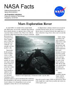
(c) Rocks: at Spirit Rover landing site

Figure 2.2: Significant landmarks (left: rover images; right: orbital images) Image Credit: NASA/JPL/University of Arizona/OSU

Mountains Mountains are very distinct. According to Webster’s online dictionary, a mountain is a landform which projects conspicuously above the surrounding terrain in a limited area. It has regions with spatial complexity, areas of high relief, and distinct changes in terrain slope (Ghosh et al., 2000). However, the view of a mountain observed from 300 m or 200 m away when a person is approaching it is quite different from the 27

view while one is on the mountain itself, which, in turn, has no similarity with what the mountain looks like from its side. Moreover, mountains are of various structural types. For example, different mountains are composed of a different number of hills and valleys. Some are steep with big slopes, while others are relatively flat. Considering these features, mountains can usually be decomposed into parts such as peaks, ridges, horizons, valleys, and watersheds. All these parts of a mountain can be described in a feature template and represented in the form of points, poly-lines, and polygons. Craters There are several different types of craters, including impact, volcanic, subsidence, and maar craters. There are more than 43,000 impact craters on the Martian surface with diameters over five kilometers (Barlow, 2000). For example, Gusev Crater, where Spirit Rover landed, has a diameter of 160 km (Grant, et al., 2004). Research on the small, simple impact craters has not been carried out in detail because of the lack of high-resolution orbital images (Golombek et al., 2006). However, all of these impact craters are important for deciphering the age and geological history of Mars. Their morphology can provide the clues to aid in understanding the nature of the Martian surface (Barlow and Sharpton, 2004) or even inform us of the possible existence of significant surface and underground water (Carr, 2004). Due to the limited rover capability of the current MER mission, the rover has only collected images of small impact craters such as Eagle, Endurance, and Victoria Craters in the Meridiani Planum and Bonneville, Missoula, and Lahontan Craters in the Gusev Crater area (Table 2.2).

28

Therefore, this research only focuses on the small craters with diameters less than one kilometer.

Location

Crater

Approximate Diameter (m)

Approximate Depth (m)

Gusev Crater landing site Meridiani Planum landing site

Bonneville Crater[1] Missoula Crater[1] Lahontan Crater[1] Eagle Crater[1] Fram Crater [2] Endurance Crater[1] Argo Crater [2] Vostok Crater [2] Erebus Crater [2] Beagle Crater [3] Emma Dean crater [2] Victoria Crater [2]

210 163 90 22 8 150 small 20 350 35 small 750

10-14 3-4 4.5 2-3 N/A 21 N/A ~0 ~0 ~1-2 N/A ~70

[1]

Ground image acquisition time (Sols) 68-86 105 118 1 84 95-315 365 399 550-750 855 929-943 951

From Grant et al., 2005 From http://www.wikipedia.com [3] From http://www.planetary.org/news/2006/0731_Mars_Exploration_Rovers_Update_Spirit.html [2]

Table 2.2 Craters in the Meridiani Planum and Gusev Crater landing sites

The classification of craters by the degree of development includes fresh crater, degraded crater, and ghost crater (Kanefsky et al., 2001). As stated on the website of the Mars

clickworkers

project

(see

http://clickworkers.arc.nasa.gov/basic-crater-

classification?), a fresh crater always has “a sharp rim, distinctive ejecta blanket, and well-preserved interior features (if any).” Some even have central peaks inside the crater. On the contrary, a degraded crater has no surrounding ejecta blanket. Its interior features are “largely or totally obliterated”. The rim is rounded or removed. A ghost crater is almost invisible through overlying deposits. For example, Erebus Crater in the Meridiani 29

Planum is a degraded crater. Erebus Crater is very old and eroded, and is almost invisible from the ground (Wikipedia, 2008b). In this dissertation, the definition of a crater is simplified to a bow-shaped structure with a rim, wall, and floor - three basic parts. The crater rim is usually higher than its surrounding terrain. The crater wall has a nearly constant slope, and the floor is relatively flat. Figure 2.3 (Di et al., 2006) is the perspective view of 3D DTM of Endurance Crater. Different colors represent various elevations at different parts of this crater model.

Crater wall Crater rim

Crater floor

Figure 2.3: Perspective view of 3D DTM of Endurance Crater

Rocks Rocks composing the Columbia Hills on the Martian surface are mainly “crustal sections that formed by volcaniclastic processes and/or impact ejecta emplacement” (Arvidson et al., 2006). Geologists usually divide rocks into groups according to their 30

various mineral compositions and developmental history. In this research, the study of rocks is used for tie point selection. Therefore, the shape of a rock is much more important for the matching of landmarks than the composition of the rock. In our definition, a rock is composed of a group of continuous surface points (red dots) and a peak (green dot) shown in Figure 2.4. The assumptions about a rock peak are that (1) the peak is the highest point of a rock, (2) it is visible from different views. Additionally, the maximum height difference between all those points should be more than 10 cm, that is, the rock identified should have a height greater than 10 cm.

Rock peak

Rock surface points

Figure 2.4: A rock

2.2 Landmark extraction Given the definitions of important landmarks above, the next step is to extract important features from different sources of images. Orbital and ground images have been processed separately in the MER mission and in previous missions (e.g. Mars Pathfinder mission). MOC and HiRISE images are taken by looking straight down from the orbit, while 360-degree high-resolution Pancam panoramic images are taken on the ground by looking around the rover with a tilt angle. Therefore, the camera models of the orbital and ground images are quite different. In addition, features shown in both kinds of 31

images also have big differences in appearance. For example, craters are usually circular looking in the MOC images, while their shape might look elliptical in the ground images. Considering the different camera geometry, methods of feature extraction are different for orbital and ground data. Because of the immense amount of image data that needs to be analyzed for presence of features, an automatic feature extraction algorithm is very important. Craters and mountains are usually selected to strengthen the correspondence between the orbital and ground images. Rocks are picked to link the correspondence of the cross sites for the ground images, because rocks are relatively small when compared with big mountains or craters. For example, a big rock two meters in width is only shown with six to seven pixels in a HiRISE image. Ground image processing with OSU MarsMapper and BA software has been well-tested in the daily MER operation at the OSU mapping and GIS Lab. Li et al. (2007c) have also developed a semi-automatic hierarchical stereo matching technique based on an image pyramid and a BA method for orbital images. DTM and orthophoto of Victoria Crater have been generated from the HiRISE stereo pair. These products have differences less than two meters in any direction when compared with those derived from the networked ground images. Victoria DTM is used for landmark modeling in this dissertation. The following subsections will give examples of automated crater detection (ACD) and rock extraction. 2.2.1 Crater detection In order to detect craters of different sizes automatically, various researchers have focused on image-based methods, which can be divided into the categories of 32

unsupervised and supervised (Bue and Stepinski, 2007). The unsupervised method is fully autonomous, which uses pattern recognition techniques such as the Hough transform or genetic algorithm (Honda and Azuma, 2000) to detect crater rims in an image, and approximates them with circular or elliptical shapes. For example, 2D edges were detected in images through an edge-detection algorithm and approximated with ellipse shapes (Leroy et al., 2001; Cheng et al., 2003). In a study by Barata et al. (2004), images were segmented through a Principle Component Analysis of statistical texture measures, and craters were detected using template matching. The supervised method trains crater detection algorithms using machine learning concepts. A set of continuously scaled templates provided detection of a range of crater sizes in synthetic terrain (Vinogradova et al., 2002). Plesko et al. (2005) developed GENetic Imagery Exploitation (GENIE) software, which applied genetic programming and support vector machines to detect craters automatically. Urbach and Stepinski (2008) used shape filters to locate candidate craters in images and classified them into craters and non-craters by supervised machine learning. These algorithms work well only for small craters or relatively simple terrain. Due to the limitations of the unsupervised and supervised algorithms, researchers (Kim and Muller, 2003; Magee et al., 2003) combined both methods to detect craters using edge processing and template matching based on local intensity values, intensity gradients, and geometric traits of images. However, image-based crater detection is not robust enough due to the lower quality of the images and the variety of crater structures. In addition to the above described image-based crater detection approaches, Michael (2003) used a constrained DTM to detect craters through Hough transform in 33

order to register the USGS MDIM 1.0 with the more precise MOLA data. Later, Bue and Stepinski (2007) developed a novel approach to detect craters based on Martian DTM data instead of images. A curvature module and a segmentation module were conducted in parallel for this approach. A topographic profile curvature was calculated in the curvature module to reflect the change in slope angle in order to detect the crater rim. The segmentation module used the flood algorithm to divide the data into small fragments without cutting through the craters. Their algorithm was tested at a heavily cratered Noachian site. Results proved that the DTM-based detection was on par with the manually compiled Barlow catalog (Barlow, 1988). This method even “outperformed Barlow catalog for small craters, but failed to identify some large, degraded craters”. However, the DTM-based method is restricted “due to the scarcity and limited resolution of planetary topography data” (Bue and Stepinski, 2007). Both the image-based and DTM-based crater detection approaches have advantages and drawbacks. They still have room for improvement. This research extracted craters using information from both the image and DTM. Following is the example of Victoria Crater extracted from a HiRISE image using edge gradient operators. Since “crater rims are often associated with the steepest gradients in the Martian landscape” (Bue and Stepinski, 2007), the two sides of crater rims usually yield a large difference in the image intensity. Therefore, the continuous edge points of a crater are the potential crater rim. First, the edge feature of this crater was detected by a Canny edge detector. As a result of this, in total, 7,375 edge points were extracted, as shown in Figure 2.5(b). Next, the shape of all the extracted edge pixels was simulated using an elliptic model by least square fitting. With this simulated elliptic model, the 34

coordinates of its center and its semi-major and semi-minor axes were calculated (Figure 2.5c). The ellipse fit quality was determined by the Ellipse-Fit-Similarity (EFS), which is defined as follows: EFS =

N 1 1 × ∑ Disk N R Ave_ellipse k =1

(2.1)

Where R Ave_ellipse is the averaged length of the semi-major and semi-minor

axes of the simulated ellipse fitting to the edge points; Disk is the Euclidean distance from the point (xk, yk) to the center of the fitted ellipse.

EFS shows how much the fitted ellipse deviates from the original edge points. As we know, the closer the EFS is approaching one the better an ellipse fits into these edge points. The result of the EFS of Victoria Crater on the HiRISE image equaled 0.9987. This value shows a good fit of the simulated ellipse. From the fitted ellipse, the semimajor and semi-minor axes were computed as 406.3 m and 382.5 m, respectively. The eccentricity of the ellipse is 0.34, which means the shape of the simulated ellipse is close to a circle. The radius was also estimated to be about 400 m by Squyres et al., (2008), and about 375 m by Li et al. (2007c). The difference is mainly caused by different processing and measuring methods.

35

North

(a) Original image

(b) Extracted crater edge points

(c) Simulated edge ellipse

Figure 2.5: Crater extraction (Victoria Crater) from HiRISE image

In addition, the Victoria DTM from USGS was read in Matlab. Then, the height was measured automatically in two different ways. The first method used the maximum height in the crater rim minus the minimum height on the crater floor. The calculated height was about 78.5 m. The second method measured the difference between the averaged height in the crater rim and that on the crater floor. The height was about 55 m. For the discussion in this dissertation, the result from the first method was used. 36

2.2.2 Rock extraction

Rocks are the primary landmarks which can be easily identified in most of the rover ground images. Usually, rocks are composed of a distinct rock peak and surface points. A peak is assumed to be the highest point always visible on a rock, no matter what the looking angle is. Therefore, rock peaks are extracted from the 3D ground points using the following assumptions: (1) they are the local maxima within a window of, for example, 50×50 cm; (2) the maximum elevation difference within the window is greater than a threshold (e.g. 10 cm); and (3) there are at least three ground points extracted within the window. These thresholds were set based on the extensive testing of Mars data in the MER 2003 mission. Based on these criteria, extraction of rock peaks can be decomposed in the following three steps: (1) interest points (e.g. rock peaks, sharp corners) extraction from stereo images using a Förstner interest operator and interest points matching using cross-correlation (Xu, 2004; Di et al., 2005); (2) dense image matching performed under the constraint of a TIN (triangulated irregular model) and dense 3D ground points calculation through space intersection of homologous image points; and (3) peak selection from the 3D ground points based on the assumptions. More details of peak extraction can be found in a study done by Li et al. (2007a). In most of the cases, the peak extraction algorithm is very successful. For example, it identified 71 peaks at Site 1200 and 95 peaks at Site 1300 of the MER-A Spirit Rover site. Figure 2.6 illustrates examples of extracted rock peaks back projected to Navcam images at Site1300.

37

Figure 2.6: Extracted rock peaks back projected to Navcam images

In addition to the rock peak, it is also important to describe the shape of a rock by its surface points and to fit these points into an analytical rock model. Through the use of an automatic searching procedure, ground points that were on the same rock were searched for in the vicinity of the peak. The procedure includes the following three steps: 1) A 3D plane is estimated using the terrain points within a certain range, e.g. 0.7 m, of the peak. In principle, the candidate rock surface points (red) are those above the plane. On the other hand, the ground points (blue) are on or very close to the plane (Figure 2.7a). The normal direction of the fitting plane is calculated and represented using a green line as shown in Figure 2.7b. A height H is calculated as the perpendicular distance from the peak to the fitted plane.

38

(a) Separation of the candidate rock surface points with the ground points after plane fitting

61.8

Up (m)

61.7 61.6 61.5 -1037

61.4

-1038 61.3 2661.5

2662

2662.5

2663

2663.5

-1039

North (m)

East (m)

(b): Plot of 3-D surface points (red) and background points (blue) with normal direction (green) Figure 2.7: Plane fitting for the background of a rock

2) Surface points are searched from the points above the fitted plane using a dynamic search range. The search range is proportional to the rock height H: kH. k varies from 0.3 to 1.7 based on a ground truth experiment where manual measurements of rocks at the Spirit site were measured and the coefficient k was calculated (Li et al., 2007a). Initially, the search from the rock peak is made in a range with the low limit radius of 0.3H. Each time a point is found, the distance from this point to the closest neighboring point is calculated. The maximum of these distances (denoted as MaxD_Neighbor) is determined. 3) An extended search is performed from each point found in the last step and within the range of MaxD_Neighbor. Therefore, the overall search radius from the peak is increased by MaxD_Neighbor. This step repeats for all points found in the last step 39

until the overall search radius reaches the upper limit of 1.7H or until no new points in the neighborhood can be added. Figure 2.8 (Li et al., 2007a) shows the rock peak and rock surface points extracted in the iterative process. The green dot is the rock peak, while the red dots are the extracted surface points.

Figure 2.8: Example of iterative surface points (red dots) extraction of a rock (green dots: rock peaks)

The above method is successfully applied to extract peaks and surface points of various types of rocks that are within 15 m from the rover, including large rocks (e.g. 0.5 m high). It is adaptive to rocks of various sizes. Examples of extracted rock peaks and surface points of other rocks are shown in Figure 2.9. The algorithm meets difficulties when dealing with a rock complex where a number of rocks stand closely together and severe occlusions block some rock peaks and surface points. However, as long as a sufficient number of rocks can be extracted and matched between two sites, the incremental BA can be achieved.

40

1

2

6

5

9

4

3

7

10

11

8

12

Figure 2.9: Example of rocks extracted with peaks (green) and surface points (red)

2.2.3 Limitations in landmark extraction

Most of the time, features such as rocks and craters are extracted successfully from the images. However, some of the limitations in the process of feature extraction are listed below: •

The quality of the image will be decreased by the image noise, which will further affect the results of feature extraction.

•

It is also difficult to extract those small and medium-sized rocks which are more than 15 meters away from the camera center. Because they only occupy several pixels in the image space, the algorithm can not extract a sufficient number of surface points for the rock to be modeled.

•

Occlusion is another problem. Some features are visible to the camera at one site but not visible in the adjacent site, a factor which is due to the scene and camera geometries. 41

2.3 Landmark modeling

With only 2D features extracted from the image space, it is not easy to match the landmarks successfully from different sources of data. In addition, the 3D information from landmark modeling needs to be combined when comparing the landmarks from cross sites or between the orbital and ground. Modeling a specific landmark is relative easy, whereas when it comes to a class of generic landmarks, there are significant difficulties in defining an ideal model. The key problems are (1) lack of specific definition of the landmark, (2) inconsistencies in resolution and viewing angle, (3) different background information, contrast, and shadow effects, and (4) occlusions. For example, before high-resolution (0.3m) MRO HiRISE was available, there was resolution discrepancy between the one to five meters MOC NA and the ground images with resolution at the centimeter level. Additionally, the shapes of the landmarks in the images may be quite different depending on the looking angle, the location of the sun, and weather. Further, even if the landmarks are similar, sometimes, it is sometimes possible that other features are occluding part of the landmark. Even when the landmarks are clearly visible, their complexity makes representation with simple descriptors difficult. Therefore, it is not an easy task to give a general model which will fit the same type of landmarks from multiple sources. Description of a landmark with single edge grouping or texture feature is not enough. In order to overcome these difficulties associated with landmark recognition, the landmark will be modeled by parts. The following gives examples of crater modeling and rock modeling.

42

2.3.1 Crater modeling

First of all, a crater has one of two basic shapes; it is either bowl-shaped or flatfloored (Jones et al., 1997). The points extracted from the edge of a crater can be used to simulate an elliptic equation, which is a shape factor. Then, the crater can be described in more detail with some dimension measure. The size of a crater can be measured with the parameters of the semi-major and semi-minor axes of the crater rim, height, and floor radius. The height information can be acquired from either MOLA DTM or stereo vision. Finally, several ratios are given as follows (Equations 2.2-2.4) to form some constraints of a crater model. Ratio1 = Length of the semi-minor axis /Length of the semi-major axis

(2.2)

Ratio2 = Floor radius /Averaged radius of the crater rim

(2.3)

Ratio3 =

Height Averaged radius of the crater rim

(2.4)

In the previous study, the height of Victoria Crater derived from its DTM is about 78.5 m. The semi-major and semi-minor axes of the crater rim are 406.3 m and 382.5 m. Therefore, the averaged radius of the rim calculated from the simulated ellipse is around 394.4 m. The floor radius is about 139 m. With these numbers, three ratios are calculated as shown in Table 2.3. These ratios, together with the crater center position, height, and radius, combine to form a feature template to describe Victoria Crater. When matching Victoria Crater from different sources, all the parameters in the feature template need to be compared. Currently, since the rover images are not sufficient to generate a 3D model of Victoria Crater, this feature template of the orbital data cannot be compared with the ground data. 43

Ratios Ratio1 Ratio2 Ratio3

Value 0.94 0.35 0.2

Table 2.3 Value of ratios from the crater model

2.3.2 Rock modeling

Rock surface points extracted from images taken at certain view points are usually distributed in the front face pointing to an observer. In order to use a symmetric model, such as a cone to model the rock, the ideal assumption is made that the peak and surface points can be used to infer the part of the rock surface which is not visible to the camera. This analytical model provides more information when compared to the above incomplete depiction with the rock peak and surface points. Therefore, a rock model with its parameters is more efficient for comparison with other rocks modeled in the same way. Based on the above-mentioned extracted rock peak and surface points, a rock can be modeled by using a 3D analytical surface (Figure A.1 in Appendix A), such as hemispheroid, semi-ellipsoid, cone, or tetrahedron (Equations A.1-A.3). More detail of the models can be found in Appendix A. The parameters of each individual rock model are estimated by a least-squares fitting using the surface points on the rock. More details on model equations, linearization, least-square solution, and fitting accuracy are given in the study by Li et al. (2007a). In the above implementation of rock modeling, the geometric shapes selected for representing the rocks are simple and idealized. An assumption is made that all of the 44

rocks stand upright on the Martian surface, i.e., the major axis is perpendicular to the XY plane. As illustrated in Figure 2.10b, the axes of some of the rocks may not be perpendicular to the XY plane. This may happen particularly in areas with big slopes. An complex rock model, considering the rock orientation angles, may be more suitable for modeling the rock, in order to reduce mismatches and produce more accurate tie points. For example, for the big rock in the middle of Figure 2.10a, using the simple models (a special case of the improved models with three orientation angles being zeros) is sufficient. For the rock shown in Figure 2.10b, in order to get more accurate rock modeling parameters, using the complex models might be better.

(a) Rocks standing in a flat horizontal plane

(b) Rocks located in steep terrain

Figure 2.10: Rocks shown on two types of terrains with different slopes

The rock models are enhanced by adding orientation angles into all the modeling equations. A single model can be transformed to a complicated model by performing three successive rotations, which can change the orientation of the reference frame from the x-y-z system of a single model to the x'-y'-z' system of a complicated model. Equations 2.5 to 2.7 describe the complex model of rocks using a hemispheroid, semiellipsoid, and cone. No analytical equation exists for the tetrahedron model. Therefore, 45

three parameters are used to represent a tetrahedron: height h, radius of the enclosing circle of the bottom triangle, and orientation angle φ of the bottom triangle. x '2 y '2 z '2 + + =1 r 2 r 2 h2

(2.5)

x' 2 y' 2 z' 2 + + =1 a 2 b2 h 2

(2.6)

x ' 2 + y ' 2 = (z '− h )

2

r2 h2

(2.7)

As shown in Equation 2.8, [x '

y ' z '] is acquired by multiplying [x T

y

z]

T

with the transformation matrix T, which is composed of three rotation matrixes (Equation 2.9, Schenk, 1999).

[x'

y ' z '] = T ⋅ [x T

0 ⎡1 ⎢ R x (α ) = 0 cos α ⎢ ⎢⎣0 − sin α

y

z ] = Rz (γ ) ⋅ R y (β ) ⋅ Rx (α ) ⋅ [x

y

z]

T

(2.8)

0 ⎤ sin α ⎥ ⎥ cos α ⎥⎦

⎡cos β R y (β ) = ⎢ 0 ⎢ ⎢⎣ sin β

0 − sin β ⎤ 1 0 ⎥ ⎥ 0 cos β ⎥⎦

⎡ cos γ Rz (γ ) = ⎢ − sin γ ⎢ ⎣⎢ 0

sin γ cos γ 0

(2.9)

0⎤ 0⎥ ⎥ 1⎦⎥

Since the semi-ellipsoid, hemispheroid, and cone models are symmetric around Z axis, only the angles α and β around the X and Y axes are actually necessary to represent the orientation of a rock. Therefore, Equation 2.10 is used to transform [x

46

y

z ] to T

[x'

y ' z '] for these three symmetric models. It is simpler than the transformation of a T

tetrahedron model, which needs three rotation angles (α, β, and γ) as illustrated by Equation 2.11. Actually, the original simple models are special cases of the new models with the three orientation angles being zeros. ⎡ x ' ⎤ ⎡cos β ⎢ y '⎥ = ⎢ 0 ⎢ ⎥ ⎢ ⎢⎣ z ' ⎥⎦ ⎢⎣ sin β

sin α ⋅ sin β cos α − sin α ⋅ cos β

⎡ x ' ⎤ ⎡ cos β ⋅ cos γ ⎢ y '⎥ = ⎢ − cos β ⋅ sin γ ⎢ ⎥ ⎢ sin β ⎣⎢ z ' ⎦⎥ ⎣⎢

− cos α ⋅ sin β ⎤ ⎡ x ⎤ ⎥⎢ y⎥ sin α ⎥⎢ ⎥ cos α ⋅ cos β ⎥⎦ ⎢⎣ z ⎥⎦

sin α ⋅ sin β ⋅ cos γ + cos α ⋅ sin γ − sin α ⋅ sin β ⋅ sin γ + cos α ⋅ cos γ − sin α ⋅ cos β

− cos α ⋅ sin β ⋅ cos γ + sin α ⋅ sin γ ⎤ ⎡ x ⎤ cos α ⋅ sin β ⋅ sin γ + sin α ⋅ cos γ ⎥ ⎢ y ⎥ ⎥⎢ ⎥ cos α ⋅ cos β ⎥⎦ ⎢⎣ z ⎥⎦

(2.10)

(2.11)

Given a hemispheroid rock model as an example (Figure 2.11), according to the equation of a hemispheroid model, the new model is similarly presented by Equation 2.5, where the parameter r is radius of the hemispheroid, and h is height. The transformation from the x-y-z coordinate system to the x'-y'-z' coordinate system is reached by rotating α and β angles along x and y axes using Equation 2.12, where the rotation matrices Rx and Ry are calculated from Equation 2.9. Putting x', y', and z' calculated from Equations 2.12 or 2.10 into Equation 2.5 and linearizing the equation, the unknown rock model parameters (h, r, α, β) are estimated using the method of Least Squares Adjustment.

47

z

z' y'

y h

x'

h x r

r

x2 y2 z2 + + =1 r2 r2 h2

x '2 y '2 z '2 + + =1 r 2 r 2 h2

(a) Simple rock models

(b) Rotated rock models

Figure 2.11: Hemispheroid rock models

[x'

y ' z '] = R y (β ) ⋅ Rx (α ) ⋅ [x T

y

z]

T

(2.12)

2.4 Results analysis of rock modeling

The initial results from crater modeling can be found in Section 2.3.1. This dissertation will mainly focus on rock modeling due to the data available. During the rock modeling process, rock surface points are first extracted in the vicinity of the peak based on a fitted plane. Next, four models (semi-ellipsoid, hemispheroid, cone, and tetrahedron) with orientation angles and without those angles are used to model specific rocks. The parameters are calculated using a Least Squares fitting. Both the simulated data and real test data are applied in both types of models. Following is a comparison of results.

2.4.1 The complex rock models with respect to the simple models using simulated data The simple models and the complex models mentioned in the last section are tested and compared using the simulated data of a hemispheroid. In all, 121 evenly distributed points are simulated in a hemispheroid with a height equal to 1 m and the 48

radius equal to 60 cm. Also, the hemispheroid is rotated along the X and Y axes from 1 to 20 degrees (20 degrees was chosen because with a slope more than 20 degrees, the terrain is too difficult to traverse). Table 2.4 shows the parameters of both the simple and the complex models. The IDs in the table refer to different rotation angles. The H column represents height, and the R column represents radius. Also, a root mean square (RMS) error is used to evaluate the fitting accuracy of a model. RMS is calculated from the differences of height z of the surface points and the fitted model height, which is shown in Equation 2.13.

∑ (z n

RMS =

− zi ,mod el )

2

i

(2.13)

i =1

n

Where zi is the height value of a surface point, zi,

model

is the height value

calculated from the fitted model using the model parameters and the known horizontal position (xi, yi) of the point.

49

ID 1 2 3 4 5 6 7 8 9 10 11 12 13 14 15 16 17 18 19 20

H (cm) 100.9 101.7 101.7 101.3 100.8 99.5 98.1 95.8 96.7 96.7 97.0 97.0 95.8 97.8 98.7 94.8 97.6 98.6 98.5 98.5

Simple model Complex model R (cm) RMS(cm) H (cm) R (cm) α(deg) β(deg) 59.7 3.2 100 60 1 1 58.8 4.3 100 60 2 2 58.5 4.5 100 60 3 3 59.3 4.6 100 60 4 4 60.1 5.3 100 60 5 5 60.3 5.5 100 60 6 6 61.0 5.9 100 60 7 7 62.3 6.0 100 60 8 8 62.6 5.6 100 60 9 9 63.0 5.3 100 60 10 10 64.0 5.4 100 60 11 11 65.3 5.5 100 60 12 12 66.2 5.6 100 60 13 13 65.1 5.1 100 60 14 14 65.6 5.0 100 60 15 15 68.7 5.7 100 60 16 16 66.4 5.0 100 60 17 17 65.2 5.6 100 60 18 18 66.0 5.7 100 60 19 19 66.9 5.9 100 60 20 20

RMS(cm) 0.0 0.0 0.0 0.0 0.0 0.0 0.0 0.0 0.0 0.0 0.0 0.0 0.0 0.0 0.0 0.0 0.0 0.0 0.0 0.0

Table 2.4 Model comparison based on the simulated dataset 1

In real cases, the extracted rock surface points are distributed only on one face of a rock. Therefore, the simple models and the complex models have also been tested using the simulated data distributed over only half of the model surface. In all, 61 evenly distributed points are simulated in half of a hemispheroid with the height equal to 1 m and the radius equal to 60 cm. Similarly to the first test, the hemispheroid is rotated along the X and Y axes from 1 to 20 degrees. The following table represents the parameters of both the simple and the complex models.

50

ID 1 2 3 4 5 6 7 8 9 10 11 12 13 14 15 16 17 18 19 20

H (cm) 100.7 101.7 101.5 102.5 102.8 102.7 102.4 106.3 104.1 103.6 102.9 104.4 103.6 103.8 102.6 102.7 102.9 102.5 102.7 103.5

Simple model Complex model R (cm) RMS(cm) H (cm) R (cm) α(deg) β(deg) RMS(cm) 60.9 3.0 100 60 1 1 0.0 61.1 3.0 100 60 2 2 0.0 61.7 3.5 100 60 3 3 0.0 61.4 4.0 100 60 4 4 0.0 62.0 4.3 100 60 5 5 0.0 63.5 4.7 100 60 6 6 0.0 65.3 4.8 100 60 7 7 0.0 63.4 4.2 100 60 8 8 0.0 63.6 5.1 100 60 9 9 0.0 64.3 5.3 100 60 10 10 0.0 65.0 4.8 100 60 11 11 0.0 65.5 4.6 100 60 12 12 0.0 66.1 4.5 100 60 13 13 0.0 66.8 4.8 100 60 14 14 0.0 67.6 4.4 100 60 15 15 0.0 68.3 4.6 100 60 16 16 0.0 69.1 4.8 100 60 17 17 0.0 70.8 5.0 100 60 18 18 0.0 71.7 5.2 100 60 19 19 0.0 71.5 5.3 100 60 20 20 0.0

Table 2.5 Model comparison based on the simulated dataset 2

Simulated data are used in both tests for the simple models and the complex models. The conclusions drawn are as follows: (1) The complex model is much more accurate than the simple model, especially when the rock has large rotation angles. (2) For the ideally simulated data, the distribution of the simulated points does not affect the results of the complex models, because the parameters (height, radius, and rotation angles) calculated are exactly the same as the real data. In addition, the RMS errors are all equal to zero.

51

(3) As for the simple models, in order to get more accurate modeling parameters, it is better to have all the surface points evenly distributed around the model. Furthermore, as the values of the rotation angles increase, the rock modeling parameters become less accurate, and the RMS errors also increase.

2.4.2 Comparison of the complex rock models with the simple models using real data Although the complex model with the rotation angles seems more accurate in describing a rock, for the real data, based on extensive tests at Sites 9600 and 9700, as well as Sites 11400 and 11493 from the MER mission data at the Spirit landing site, it was found that the parameters (e.g. height and radius) estimated from the simple models and the complex models are close. This is because the shape of a real rock is not actually a true hemisphere, ellipsoid, cone, or tetrahedron. With more unknown parameters added into the observation equation, over-fitting happens, and it is actually more difficult to get more accurate results. The test results (Tables 2.6-2.8) also show that most rocks stand upright in real world. Rocks with large rotation angles are rare. Furthermore, the simple models make the rock modeling process computationally more efficient and more robust with a limited number of surface points. Therefore, at the Spirit landing site, the simple models are sufficient for rock modeling.

52

ID Model 1 2 4 5 6 7 8 9

2 4 4 4 4 4 3 4

Simple model H R (cm) (cm) 15.6 11.1 28.5 28.6 13.8 8.9 9.4 22 40.5 41.2 22.3 25.2 25.4 35.9 14.6 19.2

RMS (cm) 3.92 4.32 4.06 1.51 4.03 4.21 4.11 3.06

Model 3 3 4 2 1 2 1 3

H (cm) 16.7 28.5 13.8 9.5 36.4 21.4 24.4 14.6

Complex model R α β (cm) (deg) (deg) 17.9 -2 -10 25.3 -10 -4 9.5 -10 -10 10.6 5 2 32.6 -10 -10 15.1 10 -4 24.8 9 7 15.5 -1 1

RMS (cm) 3.58 4.09 3.98 1.4 4.31 3.58 3.88 3.17

dH (cm) 1.1 0 0 0.1 -4.1 -0.9 -1 0

Difference dR dRMS (cm) (cm) 6.8 -0.34 -3.3 -0.23 0.6 -0.08 -11.4 -0.11 -8.6 0.28 -10.1 -0.63 -11.1 -0.23 -3.7 0.11

Table 2.6 Model comparison based on the MER-A data at Sites 9600 and 9700

ID Model 2 3 4 5 9 10 12 14 16 17 18 19

3 1 4 4 1 3 2 3 4 3 2 3

Simple model H R (cm) (cm) 18.8 25.5 22 31 28.7 31.5 32.4 43.2 13.7 18.5 10.3 16.7 11.2 7.2 9.7 24 8.2 8.8 15.3 20.5 12 21.4 9 9.3

RMS (cm) 1.91 3.3 3.52 3.56 2.63 0.93 1.8 2.34 1.97 3.33 1.13 2.08

Model 3 4 4 4 1 3 2 3 4 3 2 3

H (cm) 18.8 25.9 28.7 32.4 13.9 10.3 11.2 9.7 8.2 15.3 12 9

Complex model R α (cm) (deg) 22.9 0 37.2 -10 30.4 -10 47.9 -10 20.7 5 15.6 -5 5.7 7 14.1 -2 10.3 -10 17.3 2 20.2 -10 10.3 -10

β (deg) -1 -10 -10 -10 10 -4 -10 -10 -10 -2 6 -2

RMS (cm) 0.86 3.37 3.36 3.65 2.13 1.03 1.73 2.38 1.93 3.69 0.77 2.09

dH (cm) 0 3.9 0 0 0.2 0 0 0 0 0 0 0

Difference dR dRMS (cm) (cm) -2.6 -1.05 6.2 0.07 -1.1 -0.16 4.7 0.09 2.2 -0.5 -1.1 0.1 -1.5 -0.07 -9.9 0.04 1.5 -0.04 -3.2 0.36 -1.2 -0.36 1 0.01

Tables 2.7 Model comparison based on the MER-A data at Site 11400

ID Model 1 2 4 7 8 9 11 13 20 23 26 27 28 29

4 4 4 1 4 4 4 4 3 1 1 4 4 4

Simple model H R (cm) (cm) 14.3 19.3 14.7 17.7 19.6 22.8 15.4 12.8 16.4 43.8 19.1 30 16.9 30.6 16.5 23.6 33.8 69.4 33.5 30.6 37.2 26.2 16.5 34 28 45.1 37.9 48.2

RMS (cm) 0.9 4.08 2.06 1.34 2.81 2.69 3.2 0.85 4.24 3.64 4.13 2.84 2.81 3.63

Model 4 1 4 1 3 3 4 3 3 1 2 2 1 1

H (cm) 14.3 12.5 19.6 14.4 16.4 19.1 16.9 16.5 33.8 34.7 45.5 18.9 29.5 34.4

Complex model R α (cm) (deg) 21.5 -10 18.8 10 22.3 -10 17.5 10 40.9 1 25.9 -2 38.1 -10 13.8 0 85.1 -3 42.5 -9 30.9 6 20.6 -10 27.9 5 46.1 -10

β (deg) -10 10 -10 4 2 -1 -10 1 -7 -1 -6 10 -10 -9

RMS (cm) 2.62 3.81 1.93 2.81 2.75 3.71 2.14 1.23 3.97 3.73 4.33 2.61 2.84 3.73

dH (cm) 0 -2.2 0 -1 0 0 0 0 0 1.2 8.3 2.4 1.5 -3.5

Difference dR dRMS (cm) (cm) 2.2 1.72 1.1 -0.27 -0.5 -0.13 4.7 1.47 -2.9 -0.06 -4.1 1.02 7.5 -1.06 -9.8 0.38 15.7 -0.27 11.9 0.09 4.7 0.2 -13.4 -0.23 -17.2 0.03 -2.1 0.1

Tables 2.8 Model comparison based on the MER-A data at Site 11493

53

From the above comparison, it is concluded that the calculated orientation angle for the same rock of both sites may be quite different, although theoretically, the orientation angles should be identical. This is caused by the different looking angles of the cameras at these two sites. Sometimes, the extracted rock peaks are not the same points. They might be located on the same rock but deviate by some distance. In addition, the extracted surface points can also be different for the same rock pictured at two adjacent sites. These surface points may not have much overlapping. Even if the orientation angles of a rock were calculated at both sites, the comparison would not help much for the rock matching between the two sites. It also takes more time to do the computation in the rock modeling process. Therefore, the simple models without any orientations work better in terms of efficiency and speed than the complex models. However, it is important to add the normal direction of a fitting plane around a rock as one of the rock modeling parameters, which can be further used for rock model matching.

2.4.3 Rock modeling results Figure 2.12 (Li et al., 2007a) shows nine examples of rocks of different sizes and shapes. Each rock is modeled by using the four analytical models. Table 2.9 (Li et al., 2007a) gives the estimated model parameters of the four models for each rock, as well as the associated RMS errors of each model. The highlighted (red) RMS error of each rock is the minimum out of the four models. The corresponding model is considered the best model for that rock. For example, Rock 2 is best represented by a tetrahedron, while Rock 1 is best represented by a semi-ellipsoid. 54

Figure 2.12: Nine rocks used for modeling with four analytical models (green dots: rock peaks)

Hemispheroid model S.No

a

h

rms

Cone model r

h rms

Semi-Ellipsoid model a

b

h

rms

Tetrahedron model a

h

φ

rms

1

12.2 15.5

4.5

17.0 16.7 3.93

11.1

14.6 15.6 3.92

14.0 16.7 1.2 4.1

2

20.8 26.8

5.1

23.5 28.5 4.9

20.1

23.2 27.4 5.2

22.5 28.5 1.0 4.4

3

26.3 23.1

5.0

30.6 24.6 4.8

21.0

32.0 24.0 5.4

32.6 24.6 1.2 3.8

4

9.3

13.4

5.4

5.7

13.8 5.4

17.0

5.2 12.4 4.8

8.7

13.8 1.3 4.1

5

9.1

9.6

2.0

19.0

9.4 1.7

10.6

6.8 9.7 1.52

22.0

9.4 1.2 1.51

6

40.9 35.3

5.1

31.6 40.5 5.8

38.5

59.4 34.1 5.1

34.6 40.5 0.1 3.4

7

22.6 20.0

4.7

25.8 22.3 5.2

14.7

27.3 20.3 4.6

22.8 22.3 0.8 3.7

8

28.7 24.2

5.5

30.9 25.4 4.1

25.4

31.3 24.4 5.2

34.9 25.4 0.8 4.5

9

13.5 13.2

4.0

16.2 14.6 3.4

15.1

13.0 13.2 3.9

22.2 14.6 0.8 2.9

Table 2.9 Estimated model parameters and RMS errors (φ in radian, all others in cm) of rocks in Figure 2.12

The models of landmarks usually deviate considerably from the natural appearance. To verify the rock modeling results, Li et al. (2007a) compared the modeled parameters with the ground truth (manual measurements) of 79 rocks in the area between two adjacent sites that were 26 m apart at the Spirit landing site. Table 2.10 is an example of comparison results from four rocks shown in the top row of Figure 2.9. The big 55

difference in the height and radius is caused by the following reasons: (1) real rocks are not symmetric. A simple model may not be the best representation of the rock shape. (2) Surface points are only locate on one face of the rock. The other face is not visable and is assumed to be symmetric. On average, for the 79 rocks, the relative error between a modeled parameter and the corresponding ground truth measurement was 25.1% in height, 43.7% in radius, 57.1% in surface area, and 103.4% in volume, respectively (Table 2.11). It is obvious that height is the most reliable and thus the most comparable parameter among the four metrics. The very high difference in volume suggests that it should not be used for comparison. This verification result is important for designing the algorithm for the matching of rocks with various models.

ID

1 2 3 4

h 40.5 30.7 28.5 21.6

a 34.6 34.2 22.5 22.9

Model Results b 2r/h rms Model 1.71 3.4 Tetrahedron 41.7 2.47 8.2 Semi-Ellipsoid 1.58 4.4 Tetrahedron 2.12 2.3 Tetrahedron

Ground Truth h r 2r/h 61 62.5 2.05 22 31.0 2.82 19 28.1 2.96 23 30.8 2.68

Dif_H Dif_R

-33.6% 39.5% 50.0% -6.1%

-44.6% 22.4% -19.9% -25.6%

Table 2.10 Comparison of estimated model parameters with ground truth for 4 rocks in Figure 2.9

Parameters Height Radius Surface area Volume

Relative error (%) 25.1 43.7 57.1 103.4

Standard deviation (%) 24.1 54.6 60.6 145.5

Table 2.11 Average difference between the estimated model parameters and ground truth 56

Landmarks are one of the important factors that can be used for lander localization and rover navigation after landing (Li et al., 2006a). After landmark extraction and modeling, the next step is to match landmarks from different sources. However, the inconsistency of the viewing angle is a major challenge for achieving a correspondence between cross-site landmarks. The next chapter will present the techniques used to match the landmarks from cross rover sites.

57

CHAPTER 3 LANDMARK MATCHING In Chapter 2, the methods for landmark extraction and modeling were presented. This chapter will further describe the matching method to select cross-site tie points by comparing those landmark models automatically. This chapter is composed of three main sections. The first section will introduce the difficulties in the current work on cross-site tie points selection, where automatic matching is one of the key techniques. Next, different matching techniques will be described and compared. They include landmark modeling matching and global pattern matching. Both methods are used complementarily with each other to eliminate the potential mismatches. In the third section, the application results of the matching methods will be discussed. The results of this study show that the proposed approach functions successfully to select good cross-site tie points for mediumrange (up to 26 meters) traverse segments. In addition, a preliminary study of landmark matching between the orbital and ground images has been conducted. Some initial results are included in this chapter.

3.1 Background for the automated landmark matching Landmark matching is one of the key steps in building an image network used in bundle adjustment for rover localization. A great deal of effort has been spent on 58

matching landmarks from different sources of images including the stereo Pamcam/Navcam images from a single site and cross sites, as well as orbital images. People have been responsible for overlaying and comparing various data products including orthophotos, DTMs, footprints, anaglyph maps, and back-projection maps to interpret the image and make a decision based on their own human intelligence. In most cases, human eyes can reliably perceive landmarks and match feature patterns. This manual process is also labor-intensive for the human operator. For example, in the MER mission, the locations of the landers in the Gusev Crater and on the Meridiani Planum were identified manually by cartographic triangulation of landmarks visible in both orbital and ground images (Li et al., 2005). Additionally, in order to get a global control for the local coordinate system, ground imagery is manually referenced to MDIM and MOLA grid data through a four-stage process: 1) Pancam to DIMES and MOC using an incremental BA technique, 2) MOC to THEMIS, 3) THEMIS to MDIM, and finally, 4) MDIM to MOLA. The manual cross-site tie points selection for BA in the MER mission operation is one of the most time-consuming and difficult tasks. Landmark matching is classified into two sub-categories: cross-site and orbital to ground. Since orbital and ground integration is a complex and, as of yet, unsolved topic, this dissertation will only include some of the preliminary results at the end of this chapter. The technique for cross-site landmark matching is what will mainly be covered in this chapter. This process consists of three levels of image registration: intra-stereo, inter-stereo, and cross-site (Xu, 2004). Definitions of intra-stereo, inter-stereo, and crosssite are given in Chapter 1 (Figures 1.1 and 1.2).

59

Tie points selection from the intra- and inter-stereos at one rover site was automated based on automatic image matching using the MarsMapper software developed by the OSU Mapping and GIS Lab (Xu, 2004). However, the image matching strategy in MarsMapper cannot be used to link rocks from different sites because of the shape deformation introduced by large perspective transformations and different picturing time. For example, different parts of the rock might be visible or occluded from different sites because of different looking angles. Additionally, rock size might be measured differently due to difference in camera-object distance. Sometimes the distinct landmarks shown at one site might be absent from the adjacent site. A short traverse (e.g. 0, when r > 2h ∂V ∂V 2 2 4 2 ⎪ − = πr − πrh = πr ( r − 2h ) = ⎨= 0, when r = 2h ∂h ∂r 3 3 3 ⎪< 0, when r < 2h ⎩

(3.2)

As seen in the equation above, if the hemispheroid radius r is larger than 2h, the volume of a hemispheroid is more sensitive to h parameter. Otherwise, the volume is more sensitive to r when r is less than 2h. The calculation of the surface area of a hemispheroid model is different when the shape of a hemispheroid is in oblate or prolate condition. Equation 3.3 illustrates two representations of these conditions. ⎧ 2 πh 2 ⎛ 1 + e ⎞ ⎪⎪πr + 2e ln⎜ 1 − e ⎟, when h < r (oblate) ⎝ ⎠ S=⎨ π rh ⎪ πr 2 + sin −1 e, when h > r (prolate) ⎪⎩ e

Where e = 1 −

(3.3)

h2 r2

Usually, the surface area of a hemispheroid model is approximated by Equation 3.4. 1

⎛ r 2 p + 2r p h p ⎞ p ⎟⎟ S ≈ 2π ⎜⎜ 3 ⎝ ⎠

(3.4)

Where p = 1.6075 yields a relative error of at most 1.061%. Similarly, the first derivative of the surface area function is taken with respect to parameters of radius and height. The difference between the two derivatives is shown in 64

Equation 3.5. The derivation in Equations 3.5 and 3.6 shows ∂S / ∂r is larger than ∂S / ∂h . Therefore, the surface area of a hemispheroid is more sensitive to r. ⎛ r 2 p + 2r p h p ∂S ∂S − = 2π ⎜⎜ ∂r ∂h 3 ⎝ ⎛ r2p = 2π ⎜⎜ ⎝

⎛1 ⎞ ⎜ −1 ⎟⎟ ⎠

⎞ ⎜⎝ p ⎟⎟ ⎠

⎛ 2r 2 p −1 + 2r p −1 h p − 2r p h p −1 ⎞ ⎜⎜ ⎟⎟ 3 ⎝ ⎠ p −1 r ⎛1 ⎞ p −1 p −1 ⎜ ⎟ ( + h − r) h r p p ⎜ p −1 ⎟ 2r p −1 + 2r h ⎞ ⎝ ⎠ h ⎟⎟ >0 3 3 ⎠

r p −1 r r p −1 + h − r = r ( ) p −1 + h − r > r * 1 + h − r = h > 0, when h < r h h p −1 r r p −1 + h − r > h − r > 0, when h > r h r p −1 r p −1 + h − r = r = h > 0, when h = r h

(3.5)

(3.6)

Semi-ellipsoid Model The volume of a semi-ellipsoid is represented in Equation 3.7.

2 V = πabh 3

(3.7)

Equation 3.8 stems from the first derivatives of the volume function with respect to parameters of height, semi-major axis, and semi-minor axis. This equation demonstrates that the volume of a semi-ellipsoid is more sensitive to the smallest parameter. For example, if h is less than both a and b, the volume is more sensitive to h.

⎧ ∂V 2 ⎪ ∂h = 3 πab ⎪⎪ ∂V 2 = πbh ⎨ ⎪ ∂a 3 ⎪ ∂V = 2 πah ⎪⎩ ∂b 3

(3.8)

The surface area of a semi-ellipsoid model is shown in Equation 3.9.

65

⎛ ⎞ bh 2 S = π ⎜⎜ h 2 + F (θ , m ) + b a 2 − h 2 E (θ , m )⎟⎟ a 2 − h2 ⎝ ⎠

Where m =

(3.9)

a 2 (b 2 − h 2 ) , b 2 (a 2 − h 2 )

θ = arcsin (e ) , e = 1−

h2 , a2

and F(θ , m) and E(θ , m) are the incomplete elliptic integrals of the first and second kind.

The surface area is approximated by Equation 3.10. 1

⎛ a pb p + a ph p + b ph p ⎞ p ⎟⎟ S ≈ 2π ⎜⎜ 3 ⎝ ⎠

(3.10)

Where p = 1.6075 yields a relative error of at most 1.061%. In the same way, the first derivative of the surface area function is taken with respect to parameters of height, semi-major axis, and semi-minor axis. From Equation 3.11, the conclusion is that the surface area of a semi-ellipsoid is more sensitive to the smallest parameter. For example, if h is less than both a and b, the surface area is more sensitive to h. ⎛1 ⎞ ⎧ p p p p p p ⎜⎜ p −1 ⎟⎟ p −1 p ⎝ ⎠⎛ h ⎛ ⎞ S a b a h b h a + h p −1b p ⎞ ∂ + + ⎪ = 2π ⎜ ⎟ ⎜ ⎟⎟ ⎜ ⎟ ⎜ ⎪ ∂h 3 3 ⎝ ⎠ ⎝ ⎠ ⎪ ⎛1 ⎞ ⎜ −1 ⎟ ⎪⎪ ∂S ⎛ a p b p + a p h p + b p h p ⎞ ⎜⎝ p ⎟⎠ ⎛ a p −1b p + a p −1h p ⎞ ⎟⎟ ⎜⎜ ⎟⎟ ⎨ = 2π ⎜⎜ 3 3 ⎠ ⎝ ⎠ ⎝ ⎪ ∂a ⎛1 ⎞ ⎪ ⎜ − 1 ⎟ ⎟ p p p p p p ⎜ p −1 p p −1 p ⎪ ∂S = 2π ⎛⎜ a b + a h + b h ⎞⎟ ⎝ p ⎠ ⎛⎜ b a + b h ⎞⎟ ⎜ ⎟ ⎜ ⎟ ⎪ ∂b 3 3 ⎝ ⎠ ⎝ ⎠ ⎪⎩

66

(3.11)

Cone Model The volume of a cone model is shown in Equation 3.12.

1 V = πr 2h 3

(3.12)

Similarly, the first derivative of the volume function is taken with respect to parameters of radius and height, respectively. The difference between the two derivatives is shown in Equation 3.13. It concludes that the volume of a cone is more sensitive to h parameter when r is larger than 2h; while the volume is more sensitive to r as r is less than 2h.

⎧> 0, if r < 2h ∂V ∂V 2 1 2 1 ⎪ − = πrh − πr = πr ( 2h − r ) = ⎨= 0, if r = 2h ∂r ∂h 3 3 3 ⎪⎩< 0, if r > 2h

(3.13)

The calculation of the surface area of a cone model is shown in Equation 3.14. S = πr r 2 + h 2

(3.14)

The first derivative of the surface area function is taken with respect to the parameters of radius and height. The difference between the two derivatives shown in Equation 3.15 demonstrates that ∂S / ∂r is larger than ∂S / ∂h . Therefore, the surface area of a cone is more sensitive to r. ∂S ∂S πr 2 πrh − = π r2 + h2 + − 2 2 ∂r ∂h r +h r2 + h2 πr ( r − h ) = π r2 + h2 + r2 + h2 π ( r 2 + h 2 + r 2 − rh ) = r2 + h2 π ( r 2 + ( h − r ) 2 + rh ) >0 = r2 + h2

67

(3.15)

Tetrahedron Model No analytical equation exists for the tetrahedron model. Therefore, three parameters are used to represent a tetrahedron: height (h), radius (r) of the enclosing circle of the bottom triangle, and orientation angle (φ) of the bottom triangle. The volume and surface area of a tetrahedron model are shown in Equation 3.16 and Equation 3.17.

V=

1 1 Ah = r 2h 3 4

Where A =

S=

(3.16)

3 2 r 4

3 3 r r 2 + 4h 2 4

(3.17)

By taking the first derivatives of the volume and surface area functions with respect to the parameters of height and radius, respectively, Equation 3.18 and Equation 3.19 are deduced.

⎧> 0, if r > 2h 1 ∂V ∂V 1 2 1 ⎪ − = r − rh = r * ( r − 2h ) = ⎨= 0, if r = 2h 2 4 ∂h ∂r 4 ⎪< 0, if r < 2h ⎩ ∂S ∂S 3 3 2 3 3 − = r + 4h 2 + 4 ∂r ∂h 4 = = =

r2 r + 4h 2

2

−

3 3 2 3 3r 2 − 12 3rh r + 4h 2 + 4 4 r 2 + 4h 2 3 3 ( r 2 + 4h 2 + r 2 − 4rh )

(3.18)

3 3rh r 2 + 4h 2

(3.19)

4 r 2 + 4h 2 3 3 ( r 2 + ( 2h − r ) 2 ) 4 r 2 + 4h 2

>0

Further, it is concluded that if r is larger than 2h, the volume of a tetrahedron is more sensitive to h. Otherwise, if r is less than 2h the volume is more sensitive to r 68

(Equation 3.18). On the contrary, the surface area of a tetrahedron is always more sensitive to r because ∂S / ∂r is larger than ∂S / ∂h (Equation 3.19). Two conclusions are drawn from the analysis of parameter sensitivity for these four models (Table 3.2). The first is that hemispheroid, cone, and tetrahedron models have some similarities in parameter sensitivity. The volumes of these models are more sensitive to h when r is larger than 2h; otherwise, the volume is more sensitive to r when r is less than 2h. In addition, the surface area of these three models is more sensitive to r. Unlike the first conclusion, the second finding is that both the volume and surface area of a semi-ellipsoid model are more sensitive to the smallest parameter. In the test at the MER-A sites, most of the rock models calculated have r parameter less than twice of h parameter. Therefore, both volume and surface area of the hemispheroid, cone, and tetrahedron are more sensitive to the r parameter.

Models / Sensitivity Volume Surface area Hemispheroid, Cone, more sensitive to h, when r>2h more sensitive to r Tetrahedron more sensitive to r, when r100°) increase.

•

When six or nine well-distributed landmarks are selected, the 1% error limit is reachable if the traverse length is less than 25 m. The relative localization error increases as the traverse length and the convergence angle (>80°) increase.

•

The relative localization error is proportional to the traverse length under the condition of the same number of landmarks selected. The relative localization error also increases if the convergence angle is too small or too big.

104

Relative Localization Error with Three Landmarks (Navcam) 0.74

0.72

Relative Error (%)

0.7

0.68

0.66

0.64

0.62

0.6 20

40

(a) Two landmarks 0.52

0.45

0.5

0.44 Relative Error (%)

Relative Error (%)

0.46

0.48

0.46

0.43 0.42

0.44

0.41

0.42

0.4

60 80 100 120 Convergence Angle (degree)

140

160

(c) Four landmarks

0.39 20

40

60 80 100 120 Convergence Angle (degree)

140

(d) Six landmarks

Relative Localization Error with Nine Landmarks (Navcam) 0.4 0.39 0.38

Relative Error (%)

0.37 0.36 0.35 0.34 0.33 0.32 0.31 0.3 20

40

60 80 100 120 Convergence Angle (degree)

160

(b) Three landmarks

0.54

40

140

Relative Localization Error with Six Landmarks (Navcam)

Relative Localization Error with Four Landmarks (Navcam)

0.4 20

60 80 100 120 Convergence Angle (degree)

140

160

(e) Nine landmarks Figure 4.2: Relative localization error vs. convergence angle (distance: 7.5 m)

105

160

Relative Localization Error with Three Landmarks (Navcam) 1.5 1.45

Relative Error (%)

1.4 1.35 1.3 1.25 1.2 1.15 1.1 20

40

(a) Two landmarks (Li and Di, 2005) 0.94

0.88

0.92

0.86

0.9

0.84

Relative Error (%)

Relative Error (%)

0.9

0.88 0.86 0.84

0.82 0.8 0.78

0.82

0.76

0.8

0.74

60 80 100 120 Convergence Angle (degree)

140

160

(c) Four landmarks

0.72 20

40

60 80 100 120 Convergence Angle (degree)

140

(d) Six landmarks

Relative Localization Error with Nine Landmarks (Navcam) 0.7

0.68

Relative Error (%)

0.66

0.64

0.62

0.6

0.58

20

40

60 80 100 120 Convergence Angle (degree)

140

160

(b) Three landmarks

0.96

40

140

Relative Localization Error with Six Landmarks (Navcam)

Relative Localization Error with Four Landmarks (Navcam)

0.78 20

60 80 100 120 Convergence Angle (degree)

160

(e) Nine landmarks Figure 4.3: Relative localization error vs. convergence angle (distance: 15 m)

106

160

Relative Localization Error with Three Landmarks (Navcam) 2 1.95 1.9

Relative Error (%)

1.85 1.8 1.75 1.7 1.65 1.6 1.55 1.5 20

40

(a) Two landmarks

60 80 100 120 Convergence Angle (degree)

140

160

(b) Three landmarks Relative Localization Error with Six Landmarks (Navcam)

Relative Localization Error with Four Landmarks (Navcam)

1.25

1.35

1.3

1.2

Relative Error (%)

Relative Error (%)

1.25

1.2

1.15

1.15

1.1

1.05

1.1

1

1.05

1 20

40

60 80 100 120 Convergence Angle (degree)

140

160

(c) Four landmarks

0.95 20

40

60 80 100 120 Convergence Angle (degree)

140

(d) Six landmarks

Relative Localization Error with Nine Landmarks (Navcam) 0.94 0.92

Relative Error (%)

0.9 0.88 0.86 0.84 0.82 0.8 0.78 0.76 20

40

60 80 100 120 Convergence Angle (degree)

140

160

(e) Nine landmarks Figure 4.4: Relative localization error vs. convergence angle (distance: 20 m)

107

160

Relative Localization Error with Three Landmarks (Navcam) 2.5

2.4

Relative Error (%)

2.3

2.2

2.1

2

1.9

1.8 20

40

(a) Two landmarks 1.65

1.55

1.6

1.5

Relative Error (%)

1.45

1.5 1.45 1.4

1.4

1.35

1.3

1.35

1.25

1.3

40

60 80 100 120 Convergence Angle (degree)

140

160

(c) Four landmarks

20

40

60 80 100 120 Convergence Angle (degree)

140

(d) Six landmarks

Relative Localization Error with Nine Landmarks (Navcam) 1.15

Relative Error (%)

1.1

1.05

1

0.95

0.9 20

160

Relative Localization Error with Six Landmarks (Navcam)

1.55 Relative Error (%)

140

(b) Three landmarks

Relative Localization Error with Four Landmarks (Navcam)

1.25 20

60 80 100 120 Convergence Angle (degree)

40

60 80 100 120 Convergence Angle (degree)

140

160

(e) Nine landmarks Figure 4.5: Relative localization error vs. convergence angle (distance: 25 m)

108

160

The above analysis uses the simulated landmarks to study the relationship between rover localization accuracy with different configurations of the tie points and various traverse lengths. The 1% relative error limit is theoretically reachable at the design level with two landmarks. However, in real application, it is not easy to reach because of the real distribution of tie points. The following examples will give test results using Spirit Rover and field test data based on different traverse distance and various configurations of tie points. (1) Analysis of a traverse less than 5 m

Figure 4.6 gives the distribution of tie points for two pairs of test data at the MER-A Spirit site. Table 4.2 also provides some parameters for both pairs. The relative error is about 1.05% and 0.49% for Pair 1 and Pair 2, respectively, because the distance between the current and adjacent sites is very close (less than 5 m) for both pairs. The number of tie points is also sufficient for the BA process.

(a) Pair 1: Sites 11460 and 11489

(b) Pair 2: Sites 11460 and 11456

Figure 4.6: Distribution of tie points

109

Parameters Sites Traverse length (m) Number of tie points Relative error

Pair 1 11460 and 11489 4.6 5 1.05%

Pair 2 11460 and 11456 3.5 15 0.49%

Table 4.2 Parameters of both pairs

Assuming that there were some redundant tie points which did not contribute to the position improvement for these two pairs, two points from the original data pool were randomly chosen. Pair 1 has 10 combinations, while Pair 2 has 105 combinations. For each of the configurations with two tie points, their convergence angle and the relative localization error were calculated. The results of Pair 2 are shown in Figure 4.7. There are 40 combinations with an RE less than 5% (~0.18 m), and 65 combinations with an RE larger than 5%.

110

(a) RE < 5%

(b) RE > 5%

Figure 4.7: Relative error analysis for each of the 105 combinations of Pair 2

As we have analyzed above, theoretically, two tie points should be sufficient for traverse segments which are less than 5 m, if they have a good configuration with two cameras. However, all the REs are greater than 1% for all the 105 combinations of Pair 2, although there are eight combinations which have an RE less than 2% as shown in Figure 4.8. The common factor for these eight distributions is that they have two points located at both sides of the traverse. The convergence angle is more than 70°. This experiment concluded that small convergence angles (e.g. 20%) are shown in Figure 4.9. All these distributions have two landmarks closely chosen at one direction of 111

the traverse. The convergence angles are less than 50°. The conclusion regarding the results from Pair 1 is similar to that from Pair 2.

112

(a) RE: 1.3%

(b) RE: 1.9%

(c) RE: 1.6%

(d) RE: 1.7%

(e) RE: 1.4%

(f) RE: 1.8%

(g) RE: 1.4%

(h) RE: 1.9%

Figure 4.8: Small REs at Sites 11460 and 11456 with different distribution of two tie points (good geometry) 113

(a) RE: 49.1%

(b) RE: 42.8%

(c) RE: 31.6%

(d) RE: 31.5%

(e) RE: 26.8%

(f) RE: 23.6%

(g) RE: 22.6%

(h) RE: 20.5%

Figure 4.9: Large REs at Sites 11460 and 11456 with different distribution of two tie points (bad geometry) 114

Similarly, a configuration of three tie points and four tie points can be designed. Pair 2 has 455 different combinations for configurations of three tie points and 1365 different combinations for configurations of four tie points. Table 4.3 and Figure 4.10 give the results comparison of both configurations. From the results, we see 2% RE (7 cm) is achievable for both three tie points and four tie points configurations. The RE is more stable when four tie points are selected which have RE less than 5% (17.5 cm) in 97.9% of the combinations. In order to have less RE, it is better to select tie points which have a convergence angle of more than 100°.

Category [0, 1%] (1%, 2%] (2%, 3%] (3%, 4%] (4%, 5%] RE