1302 KSME International Journal; VoL 15 No.9, pp. 1302- I31D, 2001
Modeling and Simulation for PIG with Bypass Flow Control in Natural Gas Pipeline Tan Tien Nguyeo*, Sang Bong Kim Department of Mechanical Engineering, College of Engineering, Pukyong National University, Pusan 608-739, Korea
Hui Ryong Yoo, Yong Woo Rho Korea Gas Corporation (KOGAS), 638, It-dong, Ansan, Kyunggi-do 425-160, Korea
This paper introduces modeling and simulation results for pipeline inspection gauge (PIG) with bypass flow control in natural gas pipeline. The dynamic behaviour of the PIG depends on the different pressure across its body and the bypass flow through it. The system dynamics includes: dynamics of driving gas flow behind the PIG, dynamics of expelled gas in front of the PIG, dynamics of bypass flow, and dynamics of the PIG. The bypass flow across the PIG is treated as incompressible flow with the assumption of its Mach number smaller than 0.45. The governing nonlinear hyperbolic partial differential equations for unsteady gas flows are solved by method of characteristics (MOC) with the regular rectangular grid under appropriate initial and boundary conditions. The Runge-Kuta method is used for solving the steady flow equations to get initial flow values and the dynamic equation of the PIG. The sampling time and distance are chosen under Courant-Friedrich-Lewy (CFL) restriction. The simulation is performed with a pipeline segment in the Korea Gas Corporation (KOGAS) low pressure system, Ueijungboo -Sangye line. Simulation results show us that the derived mathematical model and the proposed computational scheme are effective for estimating the position and velocity of the PIG with bypass flow under given operational conditions of pipeline. Key Words: Pipeline Inspection Gauge (PIG), Method Of Characteristics (MOC), Bypass Flow
Nomenclature -~-------A c
: Pipe cross section [m : Wave speed [m/s]
C
: Linear damping coefficient of the PIG
Cc d dvalve
r, Ff
2
]
[Ns/m] Convection heat transfer coefficient [W/m2K] : Internal diameter of pipe Em] : Bypass valve diameter Em] : Braking force [N] : Friction force per unit pipe length [N/m] :
• Corresponding Author, E-mail:
[email protected] TEL: +82-51-620-1606; FAX: +82-51-621-1411 Department of Mechanical Engineering, College of Engineering, Pukyong National University. Pusan 608739, Korea. (Manuscript Received september 6, 2000; Revised June 4, 2001)
Ff P
Friction force between the PIG and pipeline's wall including [N] - FfPsta : Static friction force - Ff Pdyn : Dynamic friction force : The PIG driving force [N] Fp h : The opening height of valve Em] k : Pipe wall roughness Em] K : Wear factor per distance travel [N/m] Ksc : Sudden constraction loss coefficient KsE : Sudden expansion loss coefficient Ktatal : Total loss coefficient LPIG : Length of the PIG Em] m : Hydraulic mean radius of pipe Em] M : Weight of the PIG [kg] P : Flow pressure [N/m2] q : Compound rate of heat inflow per unit area of pipe wall [W /rn"] S : Perimeter of pipe [m] :
Modeling and Simulation for PIG with Bypass Flow Control in Natural Gas Pipeline
T
: Flow temperature [K]
Text
: Seabed temperature [K] : Flow velocity [m/s] : Flow velocity through valve [m/s] : Velocity of the PIG [m/s ] : Distance from pipe inlet Em] : Position of the PIG Em] : Denote flow parameter values
u tcv VPIG
x XPIG
X
Greeks r : The ratio of specific heat 2/s] II : Kinetic viscosity of flow [m S p : Flow density [kg/m ] Subscripts
L, R, M, N, S, 0, P : Denote the grid points, and 0, I
: Denote the points at inlet and outlet of pipeline
1. Introduction It is generally agreed that pipelines provide one of the most common ways and the safest means to transport large quantities of oil and gas products. Just like any other technical component, during operation, the walls of pipelines suffer a deterioration process and the pipeline conditions get worse. Pipelines can be failed with time if they are not properly maintained. One part of a maintenance procedure of pipelines is pigging them regularly to prevent the increase of their wall's roughness and the reduction of the internal diameter. The tool used for pigging is called Pipeline Inspection Gauge (PIG). There are over 350 PIGs of all types nowaday(Cordell and Vanzant, 1999). Each type of the PIG is designed for some different desired. purposes. All of the PIG is the most effective when they run at a near constant speed but will not be effective in case that they run at too high speed. The typical speeds for utility pigging are about 1-5m/s for on-stream liquids and 2-7m/s for on-stream gas(Cordell and Vanzant, 1999). So, prediction and control of the PIG velocity are very important when we operate a pipeline system. Fluid transient flows in pipelines are an interesting field in fluid mechanics and can be found
1303
in the references(White, 1999; Tannehill et al., 1997; Wylie et al., 1993; Fox, 1977). Results of research on the dynamics of the PIG in pipelines are scarcely found in the literature. Some works relating to the dynamics of the PIG without bypass flow have been reported. J. M. M. Out (1993), used Lax-Wendroff scheme for the integration of gas equations with adaptation of finite difference grid. The grid has to be continuously updated with the PIG position and the fluid values at the new grid points are estimated by interpolation. P. C. R. Lima(l999), solved this problem by using one-dimensional semi-implicit finite difference scheme. The nonlinear algebraic equations at each time step are solved by adopting Newton's method. T. T. Nguyen et aI.(2001), dealt with this problem by using MOC and regular rectangular grid for upstream and downstream flows and solved the PIG dynamic equation by using Runge-Kuta method. In the case of the PIG without bypass flow, the PIG is modelled without leakage so that upstream and downstream flows are completely separated by the PIG body. Boundary conditions at the tail and nose of the PIG for upstream and downstream flows are quite simple: the flow velocity at the PIG nose and tail equal to its velocity. In fact, there is undesired leakage flow through the PIG. Some PIGs are also designed with a flow path through their bodies. This flow is called bypass flow and varies with different pressure across the PIG. Bypass flow is not used in a sealing PIG but is often essential for an efficient cleaning operation. Bypass flow makes the PIG to slip back behind the debris that it may have scraped from the pipe wall. The purpose is to keep the debris flowing with the stream and not accumulate in front of the nose of the PIG. The presence of bypass flow reduces different pressure across the PIG and then slows down its velocity. Hence, we can also use bypass flow to control the PIG velocity. For the PIG with bypass flow, Azevedo et aI.(1996), simplified the solution under the assumption of steady state and incompressibility of flow in pipeline. This paper deals with modeling of the PIG flow in compressible, unsteady natural gas pipe-
1304
Tan Tien Nguyen. Sang Bong Kim. Hui Ryong Yoo and Yong Woo Rho
-
rncl')
L
Fig. 1 PIG flow in the natural gas pipeline line with bypass flow across its body. The PIG is driven by injected gas flow behind its tail and expelled gas flow in front of its nose. Bypass flow is controlled by opening and closing a valve placed in the PIG body. The bypass flow effects to the different pressure across the PIG and then, to its dynamic behaviour. The system dynamics includes dynamics of driving gas flow behind the PIG, dynamics of expelled gas flow in front of the PIG and movement dynamics of the PIG. The governing nonlinear hyperbolic partial differential equations of downstream and upstream gas are solved by Moe with the regular rectangular grid under appropriate initial and boundary conditions. The Runge-Kuta method is used for solving the steady flow equations to get initial flow values and the dynamics equation of the PIG.
2. Modeling
al., 1993), v. the flow of gas is quasi-steady heat flow. The unsteady flow dynamics can be modelled based on four fundamental fluid dynamic equations: continuity equation, momentum equation, state equation and energy equation. These four nonlinear hyperbolic partial differential equations are transformed to ordinary differential equations by using Moe in the following forms(Nguyen et al., 2001)
du
c dp_
+ rP dt- Ei
dx_
dt- u + c
(I)
c dp_ dx_ dt - rP dt- E2 along dt- u- c
(2)
dt
along
du
.u«:
du
dx_
dt -c dt- E3 along dt-u
(3)
where,
E =L=l_q_+ Ff 1
pm
C
pA
I) [u(rc
E = _L=l_q__ Ff C
2
pm
pA
IJ
(4)
[u(r-I) +1] c
(5) q Ffu) E 3=( r- I ) ( -m+---;r-
(6)
c=/rPp
(7)
q=Cc(TeXl- T)
(8)
A
The scheme of the PIG flow in pipeline with bypass flow is given in Fig . 1. We assume that the PIG is designed with the central bypass hole and the velocity of the PIG is controlled by controlling the bypass flow according to opening and closing the valve. 2.1 Gas flow model 2.1.1 Governing dynamics equations We assume for the natural gas flow in the pipeline as shown in Fig. I. i. the natural gas is ideal and one phase , ii. pipeline internal diameter is constant, iii. the pipe center line is in a horizontal or near horizontal line to ignore the effect of gravity , iv. the friction factor is a function of wall roughness and Reynolds number. Steady state values are used in transient calculations(Wylie et
m=S Ff=Ff(k, Re) The value of friction force, Fr, can be calculated as shown in the reference(Fox, 1977). The fluid variables p, u or p must be solved at each location x and time t. The sampling distance, L1x, and the sampling time, L1t, are chosen under the CFL stability constrain(Tannehill et al., 1997)
L1t
-----~---~-
o
L
%;.+1
t}l
!
x
I
O to get fluid velocity in the valve, Uv. Then, using Eqs. (22) and (24)-(26), we can derive the values uie«, Unose, Ptafl, and Pnose. To use Eqs. (25)-(27), the fluid parameters at point R of downstream flow and at point S of upstream flow need to be calculated first and they can be derived as the following steps: i. Calculate the flow parameters at point Nu« by linear extrapolating from two points Land N
(24)
Having established a technique for finding total loss coefficient Ktotat at any position of a closing valve in Eq. (21), it is possible to calculate pressure and velocity of fluid at the tail and nose of the PIG. From Fig. 4, using backward characteristic line at the tail of the PIG, we have
Ptail=PR+~[ -(Utail-UR)+ EIRLlt] CR (25) And using downward characteristic line, at the nose of the PIG we have
X Ntail
XNtail- XL (XN- Xd XN-XL
+ XL
(28)
ii. Calculate wave speed, cma«; at point N tail using Eq. (13) iii. Calculate the position of point R (29)
iv. Calculate the flow parameters at point R by linear interpolating from two points Land N (30)
The same steps must be done for upstream flow to find out flow parameters at point S. After finding out flow parameters at the tail of the PIG, flow parameters at point P are derived by linear interpolation from flow parameters at point P- 1 and flow parameters at the tail of the PIG. The PIG can move to the next grid space as shown in Fig. 5. In this case, two points P and P+1 need to interpolate from flow values at point P- 1 and at the tail of the PIG.
Modeling and Simulation for PIG with Bypass Flow Control in Natural Gas Pipeline
I, -
p-
I
I
__---------¢~==l--_¢_-
r,
P'
P
!'I_. --- - - - _--