Modeling and Simulation of Vehicular Networks ...

8 Modeling and Simulation of Vehicular Networks: Towards Realistic and Efficient Models Mate Boban1,2 , Tiago T. V. Vinhoza2 1 Department

of Electrical and Computer Engineering, Carnegie Mellon University 5000 Forbes Avenue, Pittsburgh, PA, 15213, USA 2 Instituto de Telecomunica¸co ˜ es, Departamento de Engenharia Electrotécnica e de Computadores Faculdade de Engenharia da Universidade do Porto, 4200-465, Porto, Portugal

USA and Portugal 1. Introduction Vehicular Ad Hoc Networks (VANETs) have been envisioned with three types of applications in mind: safety, traffic management, and commercial applications. By using wireless interfaces to form an ad hoc network, vehicles will be able to inform other vehicles about traffic accidents, hazardous road conditions and traffic congestion. Commercial applications (e.g., data exchange, audio/video communication) are envisioned to provide incentive for faster adoption of the technology. To date, the majority of VANET research efforts have relied heavily on simulations, due to prohibitive costs of employing real world testbeds. Current VANET simulators have gone a long way from the early VANET simulation environments, which often assumed unrealistic models such as random waypoint mobility, circular transmission range, or interference-free environment (Kotz et al. (2004)). However, significant efforts still remain in order to enhance the realism of VANET simulators, at the same time providing a computationally inexpensive and efficient platform for performance evaluation of VANETs. In this work, we distinguish three key building blocks of VANET simulators: – Mobility models, – Networking (data exchange) models, – Signal propagation (radio) models. Mobility models deal with realistic representation of vehicular movement, including mobility patterns (i.e., constraining vehicular mobility to the actual roadway), interactions between the vehicles (e.g., speed adjustment based on the traffic conditions) and traffic rule enforcement (e.g., intersection control through traffic lights and/or road signs). Networking models are designed to provide realistic data exchange, including simulating the medium access control (MAC) mechanisms, routing, and upper layer protocols. Signal propagation models aim at realistically modeling the complex environment surrounding the communicating vehicles, including both static objects (e.g., buildings, overpasses, hills), as well as mobile objects (other vehicles on the road). We first present the state-of-the art in vehicular mobility models and networking models and describe the most important proponents for these two aspects of VANET simulators. Then, we describe the existing signal propagation models and motivate the need for more

2 42

Theory and Applications of Ad HocApplications Networks Mobile Ad-Hoc Networks:

accurate models that are able to capture the behavior of the signal on a per-link basis, rather than relying solely on the overall statistical properties of the environment. More specifically, as shown in (Koberstein et al. (2009)), simplified stochastic radio models (e.g., free space (Goldsmith (2006)), log-distance path loss (Rappaport (1996)), two-ray ground reflection (Goldsmith (2006)), etc.), which are based on the statistical properties of the chosen environment and do not account for the specific obstacles in the region of interest, are unable to provide satisfactory accuracy for typical VANET scenarios. Contrary to this, topography-specific, highly realistic channel models (e.g., based on ray tracing (Maurer et al. (2004))) yield results that are in very good agreement with the real world. However, these models are computationally too expensive and usually bound to a specific location (e.g., a particular neighborhood in a city), thus making them impractical for extensive simulation studies. For these reasons, such models are not implemented in VANET simulators. Based on the experimental assessment of the impact of mobile obstacles on vehicle-to-vehicle communication, we point out the importance of the realistic modeling of mobile obstacles and the inconsistencies that arise in VANET simulation results in case these obstacles are omitted from the model. Motivated by this finding, we developed a novel model for incorporating the mobile obstacles (i.e., vehicles) in VANET channel modeling. A useful model that accounts for mobile obstacles must satisfy a number of requirements: accurate vehicle positioning, realistic underlying mobility model, realistic propagation characterization, and manageable complexity. The model we developed satisfies all of these requirements (Boban et al. (2011)). The proposed model accounts for vehicles as three-dimensional obstacles and takes into account their impact on the LOS obstruction, received signal power, and the packet reception rate. The algorithm behind the model allows for computationally efficient implementation in VANET simulators. Furthermore, the proposed model can easily be used in conjunction with the existing models for static obstacles to accurately simulate the entire spectrum of VANET environments with regards to both road conditions (e.g., sparse or dense vehicular networks), as well as various surroundings (including highway, suburban, and urban environments). VANET Simulation Environment

Data Exchange Modeling

Mobility Modeling

Trace-based Mobility Models

Real-world Traces

Artificial Traces

Dedicated Traffic Models

Mobility Patterns (random waypoint, Manhattan grid, roadconstrained, etc.)

Vehicle Interaction Models (lane changing, car following, accident simulation, etc.)

Signal Propagation Modeling

Deterministic Models

Traffic Rule Enforcement (intersection management, speed modeling, etc.)

Stochastic Models

Static Obstructions Modeling (e.g., road surface, buildings, hills, foliage, etc)

Mobile Obstructions Modeling (moving vehicles)

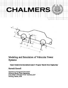
Fig. 1. Structure of VANET simulation environment

2. Mobility models Mobility models can be roughly divided in trace-based models and dedicated traffic models (Fig. 1). Trace-based models are based on a set of generated vehicular traces which are then

Modelingand andSimulation Simulation Vehicular Networks: Towards Realistic Efficient Models Modeling of of Vehicular Networks: Towards Realistic and and Efficient Models

3 43

used as an underlying mobility pattern over which the data communication is carried over. The traces can be either real world (i.e., based on mapping of the positions of vehicles) (Ferreira et al. (2009) and Ho et al. (2007)), or artificially generated using the dedicated traffic engineering tools (Naumov et al. (2006)). The advantage of trace-based models is they provide the highest level of realism achievable in VANET simulations. However, there are also several important shortcomings. Firstly, in order to collect the real world mobility traces, significant time and cost are involved. This often makes the traces collected limited with respect to both the number of the vehicles that are recorded and the region over which the recording has been made. Further this implies that there is rarely a chance to record the mobility of all the vehicles in a certain region (as it would often involve equipping each vehicle with the location devices), thus leading to a need for compensating algorithms for the non-recorded vehicles. Finally, since the traces are collected/recorded beforehand, the feedback connection from the networking model to the mobility model is not available. This is a very important shortcoming, given that a large number of proposed Intelligent Transportation System (ITS) applications carried over VANETs can affect the movement of the vehicles (this is especially the case with traffic management applications), thus rendering the trace-based models inadequate for any application with the feedback loop between the traffic and networking models. A vivid example of such application is Congested Road Notification (Bai et al. (2006)), which aids the vehicles in circumventing congested roads, thus directly affecting the mobility of the vehicles through the network communication. A characteristic that distinguishes the dedicated traffic models from the trace-based ones, capability to support the feedback loop between the mobility model and the networking model, is an important reason for adopting the more flexible dedicated traffic models. This way, the information from the networking model (e.g., a vehicle receives a traffic update advising the circumvention of a certain road) can affect the behavior of the mobility model (e.g., the vehicle takes a different route than the one initially planned). Early VANET mobility models were characterized by their simplicity and ease of implementation. For quite some time, the random waypoint mobility model (Saha & Johnson (2004)), where the vehicles move over a plane from one randomly chosen location to another, was the de facto standard for VANET simulations. However, it was shown that the overly simplified mobility models such as random waypoint are not able to model the vehicular mobility adequately (Choffnes & Bustamante (2005)). A significant step towards the realism were the simple one-dimensional freeway model and the so-called Manhattan grid model (Bai et al. (2003)), where the mobility is constrained to a set of grid-like streets which represent an urban area. Further elaboration of the mobility models was achieved by using map generation techniques, such as Voronoi graphs (Davies et al. (2006)), which constrain the movement of the vehicles to a network of artificially generated irregular streets. Recently, the most prominent mobility models (e.g., Choffnes & Bustamante (2005) and Mangharam et al. (2005)) started utilizing real world maps in order to constrain the vehicle movement to real streets based on some of the available geospatial databases (e.g., the U.S. Census Bureau’s TIGER data (U.S. Census Bureau TIGER system database (n.d.)) or the data collected in the OpenStreetMap project (Open Street Map Project (n.d.))). Furthermore, the distinction can be made with regards to the coupling between the mobility and networking and signal propagation models. On one side of the spectrum are the mobility models embedded with the networking model (Choffnes & Bustamante (2005)), which allow for a more efficient execution of the simulation. On the other side, there are mobility models which are based on the dedicated traffic simulators stemming from the traffic engineering community (e.g., SUMO - Simulation of Urban MObility (n.d.) and

4 44


CORSIM: Microscopic Traffic Simulation Model (n.d.)), which are then bidirectionally coupled ´ with the networking model (e.g., Piorkowski et al. (2008)). These types of environments are characterized by a high level of traffic simulation credibility, but often suffer from inefficiencies caused by the integration of two separate systems (Harri (2010)). Vehicle interaction (Fig. 1) includes modeling the behavior of a vehicle that is a direct consequence of the interaction with the other vehicles on the road. This includes the microscopic aspects of the impact of other vehicles, such as lane changing (Gipps (1986)) and decreasing/increasing the speed due to the surrounding traffic, as well as the macroscopic aspects, such as taking a different route due to the traffic conditions (e.g., congestion). Another important aspect of mobility modeling is traffic rule enforcement, which includes intersection management, changing the vehicle speed based on the speed limits of the roads, and generally making the vehicle obey any other traffic rules set forth on a certain highway. Even though the vehicle interaction and the enforcement of traffic rules were shown to be essential for accurate modeling of vehicular traffic (Helbing (2001)), as noted in (Harri (2010)), many of VANET mobility models have scarce support for these microscopic aspects of vehicular mobility. For this reason, significant research efforts remain in order to make these aspects of mobility models more credible, and for the research community to strive for the simulation environments that realistically model these components. With regards to the implementation approaches for the mobility models, the most prolific proponents are (Helbing (2001)): the cellular automata models (Nagel & Schreckenberg (1992)), the follow-the-leader models (e.g., car-following (Rothery (1992)) and intelligent driver model (Treiber et al. (2000))), the gas-kinetic models (Hoogendoorn & Bovy (2001)), and the macroscopic models (Lighthill & Whitham (1955)). Further classification of mobility models can be made with respect to the granularity at which the mobility is simulated, categorizing the mobility models as microscopic, mesoscopic, and macroscopic. Microscopic models are simulating the mobility at the per-vehicle level (i.e., each vehicle’s motion is simulated separately). Prominent examples of such models are the car following model (Rothery (1992)) and cellular automata models (Nagel & Schreckenberg (1992) and Tonguz et al. (2009)). Macroscopic models simulate the entire vehicular network as an entity that possesses certain physical properties. Such models can give insights into the overall statistical properties of vehicular networks (e.g., the average vehicular density, average speer, or the flow/density relationship of a given vehicular network). Examples of such models are kinematic wave models (Jin (2003)) and fluid percolation (Cheng & Robertazzi (Jul. 1989)). Mesoscopic models are simulating the mobility at the flow level, where a number of vehicles is characterized by certain averaging properties (e.g., arrival time, average speed, etc.), but the flows are distinguishable. Gas-kinetic model (Hoogendoorn & Bovy (2001)) is an example of mesoscopic models. For an extensive treatment focusing on modeling the vehicular traffic in general, we refer the reader to (Helbing (2001)), and for the overview of the mobility models used in VANET research, we refer the reader to (Harri (2010)).

3. Networking models Unlike the mobility models or signal propagation models for VANETs, which have significant differences when compared to models used in other types of mobile ad hoc networks (MANETs) (Murthy & Manoj (2004)), the networking models for VANETs are quite similar to those used in other fields of MANET research. The data models used in the current simulators, such as NS-2 (Network Simulator 2 (n.d.)), JiST/SWANS/STRAW (Choffnes & Bustamante (2005)), and NCTU-NS (Wang et al. (2003)), rely on discrete event simulation, where different


5 45

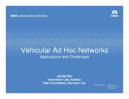
protocols of the network stack are executed based on the events triggered either by upper layer (e.g., an application sends a message to the networking protocol) or by lower layer (e.g., the link layer protocol notifies the network layer protocol about the correct reception of the message). The main difference arises in the use of a dedicated VANET protocol stack called Wireless Access in Vehicular Environments (WAVE), standardized under the IEEE 1609 working group (IEEE Trial-Use Standard for Wireless Access in Vehicular Environments (WAVE) Networking Services (Apr. 2007)). In 1999, the U.S. Federal Communications Commission (FCC) allocated 75 MHz of spectrum between 5850 - 5925 MHz for WAVE systems operating in the Intelligent Transportation System (ITS) radio service for vehicle-to-vehicle (V2V) and infrastructure-to-vehicle (V2I) communications. Similarly, the European Telecommunications Standards Institute (ETSI) has allocated 30 MHz of spectrum in the 5.9 GHz band for ITS services in August 2008, and many other countries are actively working towards standardizing the 5.9 GHz spectrum, thus allowing worldwide compatibility of WAVE devices in the future. WAVE provisions for public safety and traffic management applications. Commercial (tolling, comfort (Bai et al. (2006)), entertainment (Tonguz & Boban (2010)), etc.) services are also envisioned, creating incentive for faster adoption of the technology. The lower layers of the WAVE protocol stack are being standardized under the Dedicated short-range communications (DSRC) set of protocols (IEEE Draft Standard IEEE P802.11p/D9.0 (July 2009)). DSRC is based on IEEE 802.11 technology and is proceeding towards standardization as IEEE 802.11p. Fig. 2 shows the WAVE protocol stack. On the network layer, WAVE Short Message Protocol (WSMP) is being developed for fast and efficient message exchange in VANETs. It is planned to support both safety as well as for non-safety applications. Applications running over WSMP will directly control the physical layer characteristics (e.g., channel number and transmitter power) on a per message basis. As seen in Fig. 2, applications running over the standard TCP/IP protocol stack are also supported. Their operation is restricted to the predefined underlying physical layer characteristics, based on the application type. The applications will be divided in up to eight levels of priority, with the safety applications having the highest level of priority. The multi-channel operation (IEEE Trial-Use Standard for Wireless Access in Vehicular Environments (WAVE) - Multi-channel Operation (2006)) is aimed at providing higher availability and managing contention. Channels are divided into Control Channel (CCH) and Service Channels (SCH). WAVE devices must monitor the Control Channel (CCH) for safety application advertisements during specific intervals known as CCH intervals. CCH intervals and are specified to provide a mechanism that allows WAVE devices to operate on multiple channels while ensuring all WAVE devices are capable of receiving high-priority safety messages with high probability (IEEE Trial-Use Standard for Wireless Access in Vehicular Environments (WAVE) - Multi-channel Operation (2006)). For a tutorial on WAVE protocol stack, we refer the reader to (Uzcátegui & Acosta-Marum (2009)). Due to the relative novelty of DSRC and WAVE protocols, the majority of the widely used VANET simulators do not implement the DSRC and WAVE protocols. One exception is the NCTUNS simulation environment (Wang et al. (2003)), which implements both DSRC (IEEE 802.11p) and WAVE (IEEE 1609 set of standards) in its current version. Modeling the networking stack realistically is important for the credibility of the results obtained at each level of the protocol stack, and especially for the application level, since all the potential simulation errors from the lower layers are reflected at the application layer. To this end, it was recently shown that several stringent constraints exist in VANETs for applications (Boban et al. (2009)), and even with the optimal settings with regards to the networking model, some

6 46


Fig. 2. WAVE protocol stack. of the results reported with simplified models, especially with regards to connectivity and message reachability (e.g., Palazzi et al. (2007)) are unachievable.

4. Signal propagation models In order to adequately model the signal propagation in VANETs, appropriate models need to be developed that take into account the unique characteristics of VANET environment (e.g., high speed of the vehicles, obstruction-rich setting, specific location of the antennas, etc.). In the early days of VANET research, simple signal propagation models were utilized (e.g., unit area disk model (Gupta & Kumar (2000)), free-space path loss (Goldsmith (2006)), among others), which were carried over from MANET research. Due to the significantly different environment, these models do not provide satisfying accuracy for typical VANET scenarios (Koberstein et al. (2009)). Based on whether the model is accounting for a specific location of the objects or generalized distribution of objects in the environment, we can distinguish deterministic and stochastic models (Fig. 1). Deterministic models attempt to model the signal behavior based on the exact environment in which the vehicle is currently located, and with specific locations of the objects surrounding the vehicle (Maurer et al. (2004)). Stochastic models, on the other hand, assume a location of the surrounding objects based on a certain (often pre-defined) statistical distribution (Acosta & Ingram (2006)). Based on the approach of modeling the environment, we distinguish geometrical or non-geometrical models. Geometrical models use the concepts of computational geometry to characterize the environment by generating the possible paths or rays between the transmitting and receiving vehicle. Non-geometrical models use the higher level properties of the environment (e.g., path-loss exponent (Wang et al. (2004))) to approximate the signal power at the receiver. Furthermore, geometrical signal propagation models have to account for two types of obstructions that affect the signal: static obstructions (e.g., road surface, buildings, overpasses, hills, etc.) and mobile obstructions (moving vehicles). Numerous studies have dealt with static obstacles as the key factors affecting signal propagation (Nagel & Eichler (2008) and Giordano et al. (2010)) and proposed models for accurately quantifying the impact of static


7 47

obstacles. However, due to the nature of VANETs, where communication is often performed in V2V fashion, it is reasonable to expect that the moving vehicles will act as obstacles to the signal, often affecting the signal propagation even more than static obstacles (e.g., in case of an open road). Furthermore, the fact that the communicating entities in VANETs are vehicles exchanging data in a V2V fashion raises new challenges in signal modeling. We observe, for example, that antenna heights of both transmitter and receiver are relatively low (on top of the vehicles at best), such that other vehicles can act as obstacles for signal propagation by obstructing the LOS between the communicating vehicles. The natural conclusion is that analyzing static obstacles only is not sufficient; vehicles as moving obstacles have to be taken into account. These assumptions have been confirmed in several previous studied. Specifically, in (Otto et al. (2009)) V2V experiments were performed at 2.4 GHz frequency band in an open road environment and pointed out a significantly worse signal reception on the same road during the traffic heavy, rush hour period in comparison to a no traffic, late night period. A similar experimental V2V study presented in (Takahashi et al. (2003)) analyzed the signal propagation in “crowded” and “uncrowded” highway scenarios (depending on the number of cars currently on the road) for the 60 GHz frequency band, and reported significantly higher path loss for the crowded scenarios. Several other studies (Jerbi et al. (2007), Wu et al. (2005), Matolak et al. (2005), and Vehicle Safety Communications Project, Final Report (2006)) hint that other vehicles apart from the transmitter and receiver could be an important factor in modeling the signal propagation by obstructing the LOS between the communicating vehicles. Despite this, virtually all of the state-of-the-art VANET simulators consider the vehicles as dimensionless entities that have no influence on signal propagation (Martinez et al. (2009)). This motivated our study on the impact of vehicles as obstacles on V2V communication described in (Boban et al. (2011)) and presented in the next section.

5. Model for Incorporating Vehicles as Obstacles in VANET Simulation Environments1 5.1 Empirical measurements

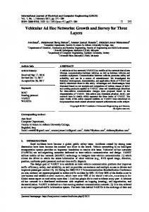
In order to quantify the impact that the vehicles have on the received signal strength, we performed experimental measurements. To isolate the effect of the obstructing vehicles, we aimed at setting up a controlled environment without other obstructions and with minimum impact of other variables (e.g., other moving objects, electromagnetic radiation, etc). For this reason, we performed experiments in an empty parking lot in Pittsburgh, PA (Fig. 3). We analyzed the received signal strength for the no obstruction, LOS case, and the non-LOS case where we introduced an obstructing vehicle (the van shown in Fig. 3) between the transmitter (Tx) and the receiver (Rx) vehicles. The received signal strength was measured for the distances of 10, 50, and 100 m between the Tx and the Rx. In case of the non-LOS experiments, the obstructing van was placed in the middle between the Tx and the Rx. We performed experiments at two frequency bands: 2.4 GHz (used by the majority of commercial WiFi devices) and 5.9 GHz (the band at which spectrum has been allocated for automotive use worldwide (IEEE Draft Standard IEEE P802.11p/D9.0 (July 2009))). For 2.4 GHz experiments, we equipped the Tx and Rx vehicles with laptops that had Atheros 802.11b/g wireless cards installed and we used 3 dBi gain omnidirectional antennas. 1 This section is based on the following paper: “Impact of Vehicles as Obstacles in Vehicular Ad Hoc c [2011] IEEE: Boban et al. (2011) Networks”, IEEE Journal on Selected Area in Communications,

8 48


RECEIVER

OBSTRUCTINGVEHICLE TRANSMITTER

ANTENNA

c [2011] IEEE Fig. 3. Experiment setup. For 5.9 GHz experiments, we equipped the Tx and Rx vehicles with NEC Linkbird-MX devices (Festag et al. (2008)), which communicate via IEEE 802.11p wireless interfaces (IEEE Draft Standard IEEE P802.11p/D9.0 (July 2009)) and we used 5 dBi gain omnidirectional antennas. In both cases, antennas were mounted on the rooftops of the Tx and Rx vehicles (Fig. 3). The dimensions of the vehicles are shown in Table 1, and the height of the antennas used in both experiments was 260 mm. The transmission power was set to 18 dBm. The Atheros wireless cards in laptops as well as IEEE 802.11p radios in LinkBird-MXs were evaluated beforehand using a real time spectrum analyzer and no significant power fluctuations were observed. The central frequency was set to 2.412 GHz and 5.9 GHz, respectively, and the channel width was 20 MHz. The data rate for 2.4 GHz experiments was 1 Mb/s, with 10 messages (140 bytes in size) sent per second using the ping command, whereas for 5.9 GHz experiments the data rate was 6 Mb/s (the lowest data rate in 802.11p for 20 MHz channel width) with 10 beacons (36 bytes in size) sent per second (Festag et al. (2008)). Each measurement was performed for at least 120 seconds, thus resulting in a minimum of 1200 data packets transmitted per measurement. We collected the per-packet Received Signal Strength Indication (RSSI) information. Figures 4a and 4b show the RSSI for the LOS (no obstruction) and non-LOS (van obstructing the LOS) measurements at 2.4 GHz and 5.9 GHz, respectively. The additional attenuation at both central frequencies ranges from approx. 20 dB at 10 m distance between Tx and Rx to 4 dB at 100 m. Even though the absolute values for the two frequencies differ (resulting mainly from the different quality radios used for 2.4 GHz and 5.9 GHz experiments), the relative trends indicate that the obstructing vehicles attenuate the signal more significantly the closer the Tx and Rx are. To provide more insight into the distribution of the received signal strength for LOS and non-LOS measurements, Fig. 5 shows the cumulative distribution function (CDF) of the RSSI measurements for 100 m in case of LOS and non-LOS at 2.4 GHz. The non-LOS case exhibits a larger variation and the two distributions are overall significantly different, thus clearly showing the impact of the obstructing van. Similar distributions were observed for other distances between the Tx and the Rx. Vehicle 2002 Lincoln LS (TX) 2009 Pontiac Vibe (RX) 2010 Ford E-250 (Obstruction) c [2011] IEEE Table 1. Dimensions of Vehicles.

Dimensions (m) Height Width Length 1.453 1.859 4.925 1.547 1.763 4.371 2.085 2.029 5.504


40 35 30 25 RSSI(dB) 20 15 10 5 0

40 35 30 25 RSSI(dB) 20 15 10 5 0

LOS Obstructed

10m

50m Distance

100m

LOS Obstructed

10m

(a) 2.4 GHz

9 49

50m Distance

100m

(b) 5.9 GHz

Fig. 4. RSSI measurements: average RSSI with and without the obstructing vehicle. c [2011] IEEE 1 0,9 0,8 0,7 0,6

CDF 0,5 0,4 0,3 0,2

100 m - No Obstruction

0,1

100 m - Obstructing Van

0 1

2

3

4

5

6

7

8

9

10 11 12 13 14 15 16

RSSI (dB)

Fig. 5. Distribution of the RSSI for 100 m in case of LOS (no obstruction) and non-LOS c [2011] IEEE (obstructing van) at 2.4 GHz.

5.2 Model analysis 5.2.1 The impact of vehicles on line of sight

In order to isolate and quantify the effect of vehicles as obstacles on signal propagation, we do not consider the effect of other obstacles such as buildings, overpasses, vegetation, or other roadside objects on the analyzed highways. Since those obstacles can only further reduce the probability of LOS, our approach leads to a best case analysis for probability of LOS. Figure 6 describes the methodology we use to quantify the impact of vehicles as obstacles on LOS in a V2V environment. Using aerial imagery (Fig. 6a) to obtain the location and length of vehicles, we devise a model that is able to analyze all possible connections between vehicles within a given range (Fig. 6b). For each link – such as the one between the vehicles designated as transmitter (Tx) and receiver (Rx) in Fig. 6b – the model determines the existence or non-existence of the LOS based on the number and dimensions of vehicles potentially obstructing the LOS (in case of the aforementioned vehicles designated as Tx and Rx, the vehicles potentially obstructing the LOS are those designated as Obstacle 1 and Obstacle 2 in Fig. 6b). The proposed model calculates the (non-)existence of the LOS for each link (i.e., between all communicating pairs) in a deterministic fashion, based on the dimensions of the vehicles and their locations. However, in order to make the model mathematically tractable, we

10 50


LOS not obstructed LOS potentially obstructed

Tx

Obstacle 1

Obstacle 2

Rx (b) Abstracted model showing possible connections

(a) Aerial photography

60% of First Fresnel Ellipsoid hi

h1 Tx

Obstacle 1 dobs1

hj

h2 d

Obstacle 2

Rx

dobs2

(c) P(LOS) calculation for a given link

Fig. 6. Model for evaluating the impact of vehicles as obstacles on LOS (for simplicity, vehicle c [2011] IEEE antenna heights (h a ) are not shown in subfigure (c)).


11 51

derive the expressions for the microscopic (i.e., per-link and per-node) and macroscopic (i.e., system-wide) probability of LOS. It has to be noted that, from the electromagnetic wave propagation perspective, the LOS is not guaranteed with the existence of the visual sight line between the Tx and Rx. It is also required that the Fresnel ellipsoid is free of obstructions ((Rappaport, 1996, Chap. 3)). Any obstacle that obstructs the Fresnel ellipsoid might affect the transmitted signal. As the distance between the transmitter and receiver increases, the diameter of the Fresnel ellipsoid increases accordingly. Besides the distance between the Tx and Rx, the Fresnel ellipsoid diameter is also a function of the wavelength. As we will show later in Section 5.3, the vehicle heights follow a normal distribution. To calculate P( LOS)ij , i.e., the probability of LOS for the link between vehicles i and j, with one vehicle as a potential obstacle between Tx and Rx (of height hi and h j , respectively), we have: h−μ P( LOS| hi , h j ) = 1 − Q (1) σ and

dobs + hi − 0.6r f + h a , (2) d where the i, j subscripts are dropped for clarity, and h denotes the effective height of the straight line that connects Tx and Rx at the obstacle location when we consider the first Fresnel ellipsoid. Furthermore, Q(·) represents the Q-function, μ is the mean height of the obstacle, σ is the standard deviation of the obstacle’s height, d is the distance between the transmitter and receiver, dobs is the distance between the transmitter and the obstacle, h a is the height of the antenna, and r f is the radius of the first Fresnel zone ellipsoid which is given by λdobs (d − dobs ) rf = , d h = ( h j − hi )

with λ denoting the wavelength. We use the appropriate λ for the proposed standard for VANET communication (DSRC), which operates in the 5.9 GHz frequency band. In our studies, we assume that the antennas are located on top of the vehicles in the middle of the roof (which was experimentally shown to be the overall optimum placement of the antenna (Kaul et al. (2007))), and we set the h a to 10 cm. As a general rule commonly used in literature, LOS is considered to be unobstructed if intermediate vehicles obstruct the first Fresnel ellipsoid by less than 40% ((Rappaport, 1996, Chap. 3)). Furthermore, for No vehicles as potential obstacles between the Tx and Rx, we get (see Fig. 6c) P( LOS| hi , h j ) =

No

∏

k =1

1−Q

hk − μk σk

,

(3)

where hk is the effective height of the straight line that connects Tx and Rx at the location of the k-th obstacle considering the first Fresnel ellipsoid, μk is the mean height of the k-th obstacle, and σk is the standard deviation of the height of the k-th obstacle. Averaging over the transmitter and receiver antenna heights with respect to the road, we obtain the unconditional P( LOS)ij P( LOS)ij =

P( LOS| hi , h j ) p(hi ) p(h j )dhi dh j ,

(4)

where p(hi ) and p(h j ) are the probability density functions for the transmitter and receiver antenna heights with respect to the road, respectively.

12 52


The average probability of LOS for a given vehicle i, P( LOS)i , and all its Ni neighbors is defined as 1 Ni P( LOS)i = P( LOS)ij (5) Ni j∑ =1 To determine the system-wide ratio of LOS paths blocked by other vehicles, we average P( LOS)i over all Nv vehicles in the system, yielding P( LOS) =

1 Nv P( LOS)i . Nv i∑ =1

(6)

Furthermore, we analyze the behavior of the probability of LOS for a given vehicle i over time. Let us denote the i-th vehicle probability of LOS at a given time t as P( LOS)it . We define the change in the probability of LOS for the i-th vehicle over two snapshots at times t1 and t2 as ΔP( LOS)i = | P( LOS)it2 − P( LOS)it1 |,

(7)

where P( LOS)it1 and P( LOS)it2 are obtained using (5). It is important to note that equations (1) to (7) depend on the distance between the node i and the node j (i.e., transmitter and receiver) in a deterministic manner. More specifically, the snapshot obtained from aerial photography provides the exact distance d (Fig. 6c) between the nodes i and j. While in our study we used aerial photography to get this information, any VANET simulator would also provide the exact location of vehicles based on the assumed mobility model (e.g., car-following (Rothery (1992)), cellular automata (Tonguz et al. (2009)), etc.), hence the distance d between the nodes i and j would still be available. This also explains why the proposed model is independent of the simulator used, since it can be incorporated into any VANET simulator, regardless of the underlying mobility model, as long as the locations of the vehicles are available. Furthermore, even though we used the highway environment for testing, the proposed model can be used for evaluating the impact of obstructing vehicles on any type of road, irrespective of the shape of the road (e.g., single or multiple lanes, straight or curvy) or location (e.g., highway, suburban, or urban2 ). 5.2.2 The impact of vehicles on signal propagation

The attenuation on a radio link increases if one or more vehicles intersect the ellipsoid corresponding to 60% of the radius of the first Fresnel zone, independent of their positions on the Tx-Rx link (Fig. 6c). This increase in attenuation is due to the diffraction of the electromagnetic waves. The additional attenuation due to diffraction depends on a variety of factors: the obstruction level, the carrier frequency, the electrical characteristics, the shape of the obstacles, and the amount of obstructions in the path between transmitter and receiver. To model vehicles obstructing the LOS, we use the knife-edge attenuation model. It is reasonable to expect that more than one vehicle can be located between transmitter (Tx) and receiver (Rx). Thus, we employ the multiple knife-edge model described in ITU-R recommendation (ITU-R (2007)). When there are no vehicles obstructing the LOS between the Tx and Rx, we use the 2 However,

to precisely quantify the impact of obstructing vehicles in complex urban environments, further research is needed to determine the interplay between the vehicle-induced obstruction and the obstruction caused by other objects (e.g., buildings, overpasses, etc.).


13 53

free space path loss model (Goldsmith (2006))3 . Single Knife-Edge The simplest obstacle model is the knife-edge model, which is a reference case for more complex obstacle models (e.g., cylinder and convex obstacles). Since the frequency of DSRC radios is 5.9 GHz, the knife-edge model theoretically presents an adequate approximation for the obstacles at hand (vehicles), as the prerequisite for the applicability of the model, namely a significantly smaller wavelength than the size of the obstacles (ITU-R (2007)), is fulfilled (the wavelength of the DSRC is approximately 5 cm, which is significantly smaller than the size of the vehicles). The obstacle is seen as a semi-infinite perfectly absorbing plane that is placed perpendicular to the radio link between the Tx and Rx. Based on the Huygens principle, the electric field is the sum of Huygens sources located in the plane above the obstruction and can be computed by solving the Fresnel integrals (Parsons (2000)). A good approximation for the additional attenuation (in dB) due to a single knife-edge obstacle Ask can be obtained using the following equation (ITU-R (2007)): ⎧ ⎪ (v − 0.1)2 + 1 + v − 0.1 ; ⎨ 6.9 + 20 log10 (8) Ask = for v > −0.7 ⎪ ⎩ 0; otherwise, √ where v = 2H/r f , H is the difference between the height of the obstacle and the height of the straight line that connects Tx and Rx, and r f is the Fresnel ellipsoid radius. Multiple Knife-Edge The extension of the single knife-edge obstacle case to the multiple knife-edge is not immediate. All of the existing methods in the literature are empirical and the results vary from optimistic to pessimistic approximations (Parsons (2000)). The method in (Epstein & Peterson (1953)) presents a more optimistic view, whereas the methods in (Deygout (1966)) and (Giovaneli (1984)) are more pessimistic approximations of the real world. Usually, the pessimistic methods are employed when it is desirable to guarantee that the system will be functional with very high probability. On the other hand, the more optimistic methods are used when analyzing the effect of interfering sources in the communications between transmitter and receiver. To calculate the additional attenuation due to vehicles, we employ the ITU-R method (ITU-R (2007)), which can be seen as a modified version of the Epstein-Patterson method, where correcting factors are added to the attenuation in order to better approximate reality. 5.3 Model requirements

The model proposed in the previous section is aimed at evaluating the impact of vehicles as obstacles using geometry concepts and relies heavily on realistic modeling of the physical environment. In order to employ the proposed model accurately, realistic modeling of the following physical properties is necessary: determining the exact position of vehicles and the inter-vehicle spacing; determining the speed of vehicles; and determining the vehicle dimensions. 3 We

acknowledge that the free space model might not be the best approximation of the LOS communication on the road. However, due to its tractability, it allows us to analyze the relationship between the LOS and non-LOS conditions in a deterministic manner.

14 54


Dataset A28 A3

Size 12.5 km 7.5 km

# vehicles 404 55

# large vehicles 58 (14.36%) 10 (18.18%)

Veh. density 32.3 veh/km 7.3 veh/km

c [2011] IEEE Table 2. Analyzed highway datasets. Determining the exact position of vehicles and the inter-vehicle spacing

The position and the speed of vehicles can easily be obtained from any currently available VANET mobility model. However, in order to test our methodology with the most realistic parameters available, we used aerial photography. This technique is used by the traffic engineering community as an alternative to ground-based traffic monitoring (McCasland, W T (1965)), and was recently applied to VANET connectivity analysis (Ferreira et al. (2009)). It is well suited to characterize the physical interdependencies of signal propagation and vehicle location, because it gives the exact position of each vehicle. We analyzed two distinct data sets, namely two Portuguese highways near the city of Porto, A28 and A3, both with four lanes (two per direction). Detailed parameters for the two datasets are presented in Table 2. For an extensive description of the method used for data collection and analysis, we refer the reader to (Ferreira et al. (2009)). Determining the speed of vehicles

For the observed datasets, besides the exact location of vehicles and the inter-vehicle distances, stereoscopic imagery was once again used to determine the speed and heading of vehicles. Since the successive photographs were taken with a fixed time interval (5 seconds), by marking the vehicles on successive photographs we were able to measure the distance the vehicle traversed, and thus infer the speed and heading of the vehicle. The measured speed and inter-vehicle spacing is used to analyze the behavior of vehicles as obstacles while they are moving. The distribution of inter-vehicle spacing for both cases can be well fitted with an exponential probability distribution. This agrees with the empirical measurements made on the I-80 interstate in California reported in (Wisitpongphan et al. (Oct. 2007)). The speed distribution on both highways is well approximated by a normal probability distribution. Table 3 shows the parameters of best fits for inter-vehicle distances and speeds. Determining the vehicle dimensions

From the photographs, we were also able to obtain the length of each vehicle accurately, however the width and height could not be determined with satisfactory accuracy due to resolution constraints and vehicle mobility. To assign proper widths and heights to vehicles, we use the data made available by the Automotive Association of Portugal (Associa¸ca˜ o Automóvel de Portugal (n.d.)), which issued an official report about all vehicles currently in circulation in Portugal. From the report we extracted the eighteen most popular personal vehicle brands which comprise 92% of all personal vehicles circulating on Portuguese roads, and consulted an online database of vehicle dimensions (Automotive Technical Data and Specifications (n.d.)) to arrive at the distribution of height and width required for our analysis. The dimensions of the most popular personal vehicles showed that both the vehicle widths and heights can be modeled as a normal random variable. Detailed parameters for the fitting process for both personal and large vehicles are presented in Table 4. For both width and height of personal vehicles, the standard error for the fitting process remained below 0.33% for both the mean and the standard deviation. The data regarding the specific types


Data for A28 Parameter Speed: normal fit mean (km/h) std. deviation (km/h) Inter-vehicle spacing : exponential fit mean (m) Data for A3 Parameter Speed: normal fit mean (km/h) std. deviation (km/h) Inter-vehicle spacing : exponential fit mean (m)

Estimate

Std. Error

106.98 21.09

1.05 0.74

51.58

2.57

Estimate

Std. Error

122.11 28.95

3.97 2.85

215.78

29.92

15 55

Table 3. Parameters of the Best Fit Distributions for Vehicle Speed and Inter-vehicle spacing. c [2011] IEEE of large vehicles (e.g., trucks, vans, or buses) currently in circulation was not available. Consequently, the precise dimension distributions of the most representative models could not be obtained. For this reason, we infer large vehicle height and width values from the data available on manufacturers’ websites, which can serve as rough dimension guidelines that show significantly different height and width in comparison to personal vehicles. 5.4 Computational complexity of the proposed model

In order to determine the LOS conditions between two neighboring nodes, we analyzed the existence of LOS in a three dimensional space, as shown in Fig. 6 and explained in the previous sections. Our model for determining the existence of LOS between vehicles and, in case of obstruction, obtaining the number and location of the obstructions, belongs to a class of computational geometry problems known as geometric intersection problems (de Berg et al. (1997)), which deal with pairwise intersections between line segments in an n-dimensional space. These problems occur in various contexts, such as computer graphics (object occlusion) and circuit design (crossing conductors), amongst others (Bentley & Ottmann (1979)). Specifically, for a given number of line segments N, we are interested in determining, reporting, and counting the pairwise intersections between the line segments. For our specific application, the line segments of interest are of two kinds: a) the LOS rays between the communicating vehicles (lines colored red in Fig. 6b); and b) the lines that compose the bounding rectangle representing the vehicles (lines colored blue in Fig. 6b). It has to be noted that the intersections of interest are only those between the LOS rays and the bounding rectangle lines, and not between the lines of the same type. Therefore, we arrive at a special case of the segment intersection problem, namely the so-called “red-blue” intersection problem. Given a set of red line segments r and a set of blue line segments b, with a total of N = r + b segments, the goal is to report all K intersections between red and blue segments, for which an efficient algorithm was presented in (Agarwal (1991)). The time-complexity of the algorithm proposed in (Agarwal (1991)), using the randomized approach of (Clarkson (1987)), is O( N 4/3 log N + K ), where K is the number of red-blue intersections, with space complexity of O( N 4/3 ). This algorithm fits our purposes perfectly, as the red segments correspond to

16 56


Personal vehicles Parameter Estimate Width: normal fit mean (cm) 175 std. deviation (cm) 8.3 Height: normal fit mean (cm) 150 std. deviation (cm) 8.4 Large vehicles Parameter Estimate Width: constant mean (cm) 250 Height: normal fit mean (cm) 335 std. deviation (cm) 8.4 c [2011] IEEE Table 4. Parameters of the Best Fit Distributions for Vehicle Width and Height. the LOS rays between the communicating vehicles and blue segments are the lines of the bounding rectangles representing the vehicles (see Fig. 6b). To assign physical values to r and b, we denote v as the number of vehicles in the system and v as the number of transmitting vehicles. The number of LOS rays results in r = Cv , where the average number of neighbors C is an increasing function of the vehicle density and transmission range. The number of lines composing the bounding vehicle rectangles can be expressed as b = 4v, since each vehicle is represented by four lines forming a rectangle (see Fig. 6b). Therefore, a more specific time-complexity bound can be written as O((Cv + 4v)4/3 log(Cv + 4v) + K ). Apart from the algorithm for determining the red-blue intersections, the rest of the proposed model consists in calculating the additional signal attenuation due to vehicles for each communicating pair. In the case of non-obstructed LOS the algorithm terminates, whereas for obstructed LOS, the red-blue intersection algorithm is used to store the number and location of intersecting blue lines (representing obstacles). The total number of intersections is given by K = gr, where g is the number of obstacles (i.e., vehicles) in the LOS path and is a subset of C. The complete algorithm for additional attenuation due to vehicles is implemented as follows. The function getIntersect(·) is based on the aforementioned red-blue line intersection algorithm (Agarwal (1991)), and has complexity O((Cv + 4v)4/3 log(Cv + 4v) + gr ), whereas the function calcAddAtten(·) is based on multiple knife-edge attenuation model described in (ITU-R (2007)) with time-complexity of O( g2 ) for each LOS ray r. It follows that the time-complexity of the entire algorithm is given by O((Cv + 4v)4/3 log(Cv + 4v) + g2 r). In order to implement the aforementioned algorithm in VANET simulators, apart from the information available in the current VANET simulators, very few additional pieces of information are necessary. Specifically, the required information pertains to the physical dimensions of the vehicles. Apart from this, the model only requires the information on the position of the vehicles at each simulation time step. This information is available in any vehicular mobility model currently in use in VANET simulators.


17 57

Algorithm 1 Calculate additional attenuation due to vehicles for i = 1 to r do [coord] = getIntersect(i ) {For each LOS ray in r, obtain the location of intersections as per (Agarwal (1991))} if size([coord]) = 0 then att = calcAddAtten([coord]) {Calculate the additional attenuation due to vehicles as per (ITU-R (2007))} else att = 0 dB {Additional attenuation due to vehicles equals zero.} end if end for

Highway A3 P( LOS) A28 P( LOS)

Highways Transmission Range (m) 100 250 500 0.8445 0.6839 0.6597 0.8213 0.6605 0.6149

c [2011] IEEE Table 5. P( LOS) for A3 and A28. 5.5 Results

We implemented the model described in previous sections in Matlab. In this section we present the results based on testing the model using the A3 and A28 datasets. We also present the results of the empirical measurements that we performed in order to characterize the impact of the obstructing vehicles on the received signal strength. We emphasize that the model developed in the paper is not dependent on these datasets, but can be used in any environment by applying the analysis presented in Section 5.2. Furthermore, the observations pertaining to the inter-vehicle and speed distributions on A3 and A28 are used only to characterize the behavior of the highway environment over time. We do not use these distributions in our model; rather, we use actual positions of the vehicles. Since the model developed in Section 5.2 is intended to be utilized by VANET simulators, the positions of the vehicles can easily be obtained through the employed vehicular mobility model. We first give evidence that vehicles as obstacles have a significant impact on LOS communication in both sparse (A3) and more dense (A28) networks. Next, we analyze the microscopic probability of LOS to determine the variation of the LOS conditions over time for a given vehicle. Then, we used the speed and heading information to characterize both the microscopic and macroscopic behavior of the probability of LOS on highways over time in order to determine how often the proposed model needs to be recalculated in the simulators, and to infer the stationarity of the system-wide probability of LOS. Using the employed multiple knife-edge model, we present the results pertaining to the decrease of the received power and packet loss for DSRC due to vehicles. Finally, we corroborate our findings on the impact of the obstructing vehicles and discuss the appropriateness of the knife-edge model by performing empirical measurements of the received signal strength in LOS and non-LOS conditions.

18 58


Average Number of Neighbors

50

LOS Not Obstructed LOS Obstructed

40

30

20

10

0

100

300 500 750 Transmission range (meters)

Fig. 7. Average number of neighbors with unobstructed and obstructed LOS on A28 c [2011] IEEE highway. 5.5.1 Probability of line of sight

Macroscopic probability of line of sight. Table 5 presents the values of P( LOS) with respect to the observed range on highways. The highway results show that even for the sparsely populated A3 highway the impact of vehicles on P( LOS) is significant. This can be explained by the exponential inter-vehicle spacing, which makes it more probable that the vehicles are located close to each other, thus increasing the probability of having an obstructed link between two vehicles. For both highways, it is clear that the impact of other vehicles as obstacles can not be neglected even for vehicles that are relatively close to each other (for the observed range of 100 m, P( LOS) is under 85% for both highways, which means that there is a non-negligible 15% probability that the vehicles will not have LOS while communicating). To confirm these results, Fig. 7 shows the average number of neighbors with obstructed and unobstructed LOS for the A28 highway. The increase of obstructed vehicles in both absolute and relative sense is evident. Microscopic probability of line of sight. In order to analyze the variation of the probability of LOS for a vehicle and its neighbors over time, we observe the ΔP( LOS)i (as defined in equation (7)) on A28 highway for the maximum communication range of 750 m. Table 6 shows the ΔP( LOS)i . The variation of probability of LOS is moderate for periods of seconds (even for the largest offset of 2 seconds, only 15% of the nodes have the ΔP( LOS)i greater than 20%). This result suggests that the LOS conditions between a vehicle and its neighbors will remain largely unchanged for a period of seconds. Therefore, a simulation time-step of the order of seconds can be used for calculations of the impact of vehicles as obstacles. From a simulation execution standpoint, the time-step of the order of seconds is quite a long time when compared with the rate of message transmission, measured in milliseconds; this enables a more efficient and scalable design and modeling of vehicles as obstacles on a microscopic, per-vehicle level. With the proper implementation of the LOS intersection model discussed in Sections 5.2 and 5.4 , the modeling of vehicles as obstacles should not induce a large overhead in the simulation execution time. 5.5.2 Received power

Based on the methodology developed in Section 5.2, we utilize the multiple knife-edge model to calculate the additional attenuation due to vehicles. We use the obtained attenuation to calculate the received signal power for the DSRC. We employed the knife-edge model for its


< 5% 100% 99% 82% 35% 31%

Time offset 1ms 10ms 100ms 1s 2s

ΔP( LOS)i in % 5-10% 10-20% 0% 0% 1% 0% 15% 3% 33% 22% 25% 29%

19 59

>20% 0% 0% 0% 10% 15%

Table 6. Variation of P( LOS)i over time for the observed range of 750 m on A28. c [2011] IEEE 1

Cumulative Distribution Function

0.9 0.8 Rx sensitivity level 0.7 0.6 0.5 0.4 0.3 0.2

Vehicles as obstacles Free Space

0.1 0 −110

−100

−90

−80

−70

−60

Received Power Level (dBm)

−50

−40

Fig. 8. The impact of vehicles as obstacles on the received signal power on highway A28. simplicity and the fact that it is well studied and often used in the literature. However, we point out that the LOS analysis and the methodology developed in Section 5.2 can be used in conjunction with any channel model that relies on the distinction between the LOS and NLOS communication (Zang et al. (2005) and Wang et al. (2004)). For the A28 highway and the observed range of 750 m, with the transmit power set to 18 dBm, 3 dBi antenna gain for both transmitters and receivers, at the 5.9 GHz frequency band, the results for the free space path loss model (Goldsmith (2006)) (i.e., not including vehicles as obstacles) and our model that accounts for vehicles as obstacles are shown in Fig. 8. The average additional attenuation due to vehicles was 9.2 dB for the observed highway. Using the minimum sensitivity thresholds as defined in the DSRC standard (see Table 7) (Standard Specification for Telecommunications and Information Exchange Between Roadside and Vehicle Systems - 5GHz Band Dedicated Short Range Communications (DSRC) Medium Access Data Rate (Mb/s) 3 4.5 6 9 12 18 24 27

Modulation BPSK BPSK QPSK QPSK QAM-16 QAM-16 QAM-64 QAM-64

Minimum sensitivity (dBm) −85 −84 −82 −80 −77 −70 −69 −67

c [2011] IEEE Table 7. Requirements for DSRC Receiver Performance.

20 60

Theory and Applications of Ad HocApplications Networks Mobile Ad-Hoc Networks: 1

Packet sucess rate

0.9

0.8

0.7

0.6

0.5

0.4 100

3Mb/s − obstacles 6Mb/s − obstacles 12Mb/s − obstacles 3Mb/s − free space 6Mb/s − free space 12Mb/s − free space

250

375 500 Transmission Range (m)

625

750

Fig. 9. The impact of vehicles as obstacles on packet success rate for various DSRC data rates c [2011] IEEE on A28 highway. Control (MAC) and Physical Layer (PHY) Specifications (Sep. 2003)), we calculate the packet success rate (PSR, defined as the ratio of received messages to sent messages) as follows. We analyze all of the communicating pairs within an observed range, and calculate the received signal power for each message. Based on the sensitivity thresholds presented in Table 7, we determine whether a message is successfully received. For the A28 highway, Fig. 9 shows the PSR difference between the free space path loss and the implemented model with vehicles as obstacles for rates of 3, 6, and 12 Mb/s. The results show that the difference is significant, as the percentage of lost packets can be up to 25% higher when vehicles are accounted for. These results show that not only do the vehicles significantly decrease the received signal power, but the resulting received power is highly variable even for relatively short distances between the communicating vehicles, thus calling for a microscopic, per-vehicle analysis of the impact of obstructing vehicles. Models that try to average the additional attenuation due to vehicles could fail to describe the complexity of the environment, thus yielding unrealistic results. Furthermore, the results show that the distance itself can not be solely used for determining the received power, since even the vehicles close by can have a number of other vehicles obstructing the communication path and therefore the received signal power becomes worse than for vehicles further apart that do not have obstructing vehicles between them. 5.6 Discussion

In this section, we describe the impact that the obtained results have on various aspects of V2V communication modeling, ranging from physical to application layer to the realism of VANET simulators. 5.6.1 Impact on signal propagation modeling

The results presented in this paper clearly indicate that vehicles as obstacles have a significant impact on signal propagation; therefore, in order to properly model V2V communication, it is imperative that vehicles as obstacles are accounted for. Furthermore, the effect of vehicles as obstacles cannot be neglected even in the case of relatively sparse vehicular networks, as one of the two analyzed highway datasets showed (namely, the dataset collected on the A3 highway). Therefore, previous efforts pertaining to signal propagation modeling in V2V communication which do not account for vehicles as obstacles, can be deemed as optimistic in overestimating the received signal power level.


21 61

5.6.2 Impact on data link layer

Neglecting vehicles as obstacles on the physical layer has profound effects on the performance of upper layers of the communication stack. The effects on the data link layer are twofold: a) the medium contention is overestimated in models that do not include vehicles as obstacles in the calculation, thus potentially representing a more pessimistic situation than the real-world with regards to contention and collision; and b) the network reachability is bound to be overestimated, due to the fact that the signal is considered to reach more neighbors and at a higher power than in the real world. These results have important implications for vehicular Medium Access Control (MAC) protocol design; MAC protocols will have to cope with an increased number of hidden vehicles due to other vehicles obstructing them. 5.6.3 Impact on the design of routing protocols

If vehicles as obstacles are not accounted for, the impact on routing protocols is represented by an overly optimistic hop count; in the process of routing, next hop neighbors are selected that are actually not within the reach of the current transmitter, thus inducing an unrealistic behavior of the routing protocol, as the message is considered to reach the destination with a smaller number of hops than it is actually required. As an especially important class of routing protocols, safety messaging protocols, are often modeled and evaluated using distance information only. As our results have shown, not accounting for vehicles as obstacles in such calculations results in the overestimation of the number of reachable neighbors, which yields unrealistic results with regards to network reachability and message penetration rate. Therefore, it is extremely important to account for vehicles as obstacles in V2V, especially since safety applications running over such protocols require that practically all vehicles receive the message, thus posing very stringent requirements on the routing protocols. For these reasons, it is more beneficial to design routing protocols that rely primarily on the received signal strength instead of the geographical location of vehicles, since this would ensure that the designated recipient is actually able to receive the message. However, even with smart protocols that are able to properly evaluate the channel characteristics between the vehicles, in case of lower market penetration rates of the communicating equipment, the vehicles that are not equipped could significantly hinder the communication between the equipped vehicles; this is another aspect of routing protocol design that is significantly affected by the impact of vehicles as obstacles in V2V communication. Similarly, the results suggest that, where available, vehicle-to-infrastructure (V2I) communication (where vehicles are communicating with road side equipment) should be favored instead of V2V communication; since the road side equipment is supposed to be placed in lamp posts, traffic lights, or on the gantries above the highways such as the one in the Fig. 6a), all of which are located 3-6 meters above ground level, other vehicles as obstacles would impact the LOS much less than in the case of V2V communication. Therefore, similarly to differentiating vehicles with regards to their dimensions, routing protocols would benefit from being able to differentiate between the road side equipment and vehicles. 5.6.4 Impact on VANET simulations

VANET simulation environments have largely neglected the modeling of vehicles as obstacles in V2V communication. Results presented in this paper showed that the vehicles have a significant impact on the LOS, and in order to realistically model the V2V communication in simulation environments, vehicles as obstacles have to be accounted for. This implies that

22 62


the models that relied on the simulation results that did not account for vehicles as obstacles have been at best producing an optimistic upper bound of the results that can be expected in the real world. In order to improve the realism of the simulators and to enable the implementation of a scalable and realistic framework for describing the vehicles as obstacles in V2V communication, we proposed a simple yet realistic model for determining the probability of LOS on both macroscopic and microscopic level. Using the results that proved the stationarity of the probability of LOS, we showed that the average probability of LOS does not change over time if the vehicle arrival rate remains constant. Furthermore, over a period of seconds, the LOS conditions remain mostly constant even for the microscopic, per-vehicle case. This implies that the modeling of the impact of vehicles as obstacles can be performed at the rate of seconds, which is two to three orders of magnitude less frequent than the rate of message exchange (most often, messages are exchanged on a millisecond basis). Therefore, with the proper implementation of the proposed model, the calculation of the impact of vehicles on LOS should not induce a large overhead in the simulation execution time.

6. Conclusions We discussed the state-of-the-art in VANET modeling and simulation, and described the building blocks of VANET simulation environments, namely the mobility, networking and signal propagation models. We described the most important models for each of these categories, and we emphasized that several areas are not optimally represented in state-of-the-art VANET simulators. Namely, the vehicle interaction and traffic rule enforcement models in most current simulators leave a lot to be desired, and the lack of WAVE and DSRC protocol implementation in the simulators is also a fact for most simulators. Finally, we pointed out that the models for moving obstacles are lacking in modern simulators, and we described our proposed model for vehicles as physical obstacles in VANETs as follows. First, using the experimental data collected in a measurement campaign, and by utilizing the real world data collected by means of stereoscopic aerial photography, we showed that vehicles as obstacles have a significant impact on signal propagation in V2V communication; in order to realistically model the communication, it is imperative that vehicles as obstacles are accounted for. The obtained results point out that vehicles are an important factor in both highway and urban, as well as in sparse and dense networks. Next, we characterized the vehicles as three-dimensional objects that can obstruct the LOS between the communicating pair. Then, we modeled the vehicles as physical obstacles that attenuate the signal, which allowed us to determine their impact on the received signal power, and consequently on the packet error rate. The presented model is computationally efficient and, as the results showed, can be updated at a rate much lower than the message exchange rate in VANETs. Therefore, it can easily be implemented in any VANET simulation environment to increase the realism.

7. References Acosta, G. & Ingram, M. (2006). Model development for the wideband expressway vehicle-to-vehicle 2.4 GHz channel, IEEE Wireless Communications and Networking Conference, 2006. WCNC 2006., Vol. 3, pp. 1283–1288. Agarwal, P. K. (1991). Intersection and Decomposition Algorithms for Planar Arrangements, Cambridge University Press. Associa¸ca˜ o Automóvel de Portugal (n.d.).


23 63

URL: http://www.acap.pt/ Automotive Technical Data and Specifications (n.d.). URL: http://www.carfolio.com/ Bai, F., Elbatt, T., Hollan, G., Krishnan, H. & Sadekar, V. (2006). Towards characterizing and classifying communication-based automotive applications from a wireless networking perspective, 1st IEEE Workshop on Automotive Networking and Applications (AutoNet) . Bai, F., Sadagopan, N. & Helmy, A. (2003). IMPORTANT: a framework to systematically analyze the impact of mobility on performance of routing protocols for adhoc networks, INFOCOM 2003. Twenty-Second Annual Joint Conference of the IEEE Computer and Communications Societies. IEEE 2: 825–835 vol.2. Bentley, J. & Ottmann, T. (1979). Algorithms for reporting and counting geometric intersections, Computers, IEEE Transactions on C-28(9): 643–647. Boban, M., Tonguz, O. & Barros, J. (2009). Unicast communication in vehicular ad hoc networks: a reality check, IEEE Communications Letters 13(12): 995–997. Boban, M., Vinhoza, T. T. V., Barros, J., Ferreira, M. & Tonguz, O. K. (2011). Impact of Vehicles as Obstacles in Vehicular Ad Hoc Networks, IEEE Journal on Selected Areas in Communications 29(1): 15–28. Cheng, Y. & Robertazzi, T. (Jul. 1989). Critical Connectivity Phenomena in Multihop Radio Models, IEEE Transactions on Communications 37(7): 770–777. Choffnes, D. R. & Bustamante, F. E. (2005). An integrated mobility and traffic model for vehicular wireless networks, VANET ’05: Proceedings of the 2nd ACM international workshop on Vehicular ad hoc networks, ACM, New York, NY, USA, pp. 69–78. Clarkson, K. (1987). New applications of random sampling in computational geometry, Discrete and Computational Geometry 2: 195–222. CORSIM: Microscopic Traffic Simulation Model (n.d.). URL: http://www-mctrans.ce.ufl.edu/featured/TSIS/ Davies, J. J., Beresford, A. R. & Hopper, A. (2006). Scalable, distributed, real-time map generation, IEEE Pervasive Computing 5(4): 47–54. de Berg, M., van Kreveld, M., Overmars, M. & Schwarzkopf, O. (1997). Computational Geometry Algorithms and Applications, Springer-Verlag. Deygout, J. (1966). Multiple knife-edge diffraction of microwaves, IEEE Transactions on Antennas and Propagation 14(4): 480–489. Epstein, J. & Peterson, D. W. (1953). An experimental study of wave propagatin at 850MC, Proceedings of the IRE 41(5): 595–611. Ferreira, M., Conceiça˜ o, H., Fernandes, R. & Tonguz, O. K. (2009). Stereoscopic Aerial Photography: An Alternative to Model-Based Urban Mobility Approaches, Proceedings of the Sixth ACM International Workshop on VehiculAr Inter-NETworking (VANET 2009), ACM New York, NY, USA. Festag, A., Baldessari, R., Zhang, W., Le, L., Sarma, A. & Fukukawa, M. (2008). Car-2-x communication for safety and infotainment in europe, NEC Technical Journal 3(1). Giordano, E., Frank, R., Pau, G. & Gerla, M. (2010). Corner: a realistic urban propagation model for vanet, WONS’10: Proceedings of the 7th international conference on Wireless on-demand network systems and services, IEEE Press, Piscataway, NJ, USA, pp. 57–60. Giovaneli, C. L. (1984). An analysis of simplified solutions for multiple knife-edge diffraction, IEEE Transactions on Antennas and Propagation 32(3): 297–301. Gipps, P. G. (1986). A model for the structure of lane-changing decisions, Transportation

24 64


Research Part B: Methodological 20(5): 403–414. Goldsmith, A. J. (2006). Wireless Communications, Cambridge University Press. Gupta, P. & Kumar, P. (2000). The Capacity of Wireless Networks, IEEE Transactions on Information Theory 46(2): 388–404. Harri, J. (2010). Vehicular mobility modeling for vanet, VANET Vehicular Applications and Inter-Networking Technologies, Wiley, pp. 107–152. Helbing, D. (2001). Traffic and related self-driven many-particle systems, Rev. Mod. Phys. 73(4): 1067–1141. Ho, I. W., Leung, K. K., Polak, J. W. & Mangharam, R. (2007). Node connectivity in vehicular ad hoc networks with structured mobility, 32nd IEEE Conference on Local Computer Networks, LCN 2007. pp. 635–642. Hoogendoorn, S. & Bovy, P. (2001). Generic gas-kinetic traffic systems modeling with applications to vehicular traffic flow. IEEE Draft Standard IEEE P802.11p/D9.0 (July 2009). Technical report. IEEE Trial-Use Standard for Wireless Access in Vehicular Environments (WAVE) - Multi-channel Operation (2006). IEEE Std 1609.4-2006 pp. c1–74. IEEE Trial-Use Standard for Wireless Access in Vehicular Environments (WAVE) - Networking Services (Apr. 2007). IEEE Std 1609.3-2007 pp. c1–87. ITU-R (2007). Propagation by diffraction, Recommendation P.526, International Telecommunication Union Radiocommunication Sector, Geneva. Jerbi, M., Marlier, P. & Senouci, S. M. (2007). Experimental assessment of V2V and I2V communications, Proc. IEEE Internatonal Conference on Mobile Adhoc and Sensor Systems (MASS 2007), pp. 1–6. Jin, W. (2003). Kinematic wave models of network vehicular traffic. Ph.D. Dissertation, UC Davis. Kaul, S., Ramachandran, K., Shankar, P., Oh, S., Gruteser, M., Seskar, I. & Nadeem, T. (2007). Effect of antenna placement and diversity on vehicular network communications, Proc. IEEE SECON., pp. 112–121. Koberstein, J., Witt, S. & Luttenberger, N. (2009). Model complexity vs. better parameter value estimation: comparing four topography-independent radio models, Simutools ’09: Proceedings of the 2nd International Conference on Simulation Tools and Techniques, ICST (Institute for Computer Sciences, Social-Informatics and Telecommunications Engineering), ICST, Brussels, Belgium, Belgium, pp. 1–8. Kotz, D., Newport, C., Gray, R. S., Liu, J., Yuan, Y. & Elliott, C. (2004). Experimental evaluation of wireless simulation assumptions, Proc. ACM MSWiM ’04, ACM, New York, NY, USA, pp. 78–82. Lighthill, M. J. & Whitham, G. B. (1955). On Kinematic Waves. II. A Theory of Traffic Flow on Long Crowded Roads, Royal Society of London Proceedings Series A 229: 317–345. Mangharam, R., Weller, D. S., Stancil, D. D., Rajkumar, R. & Parikh, J. S. (2005). Groovesim: a topography-accurate simulator for geographic routing in vehicular networks, VANET ’05: Proceedings of the 2nd ACM international workshop on Vehicular ad hoc networks, ACM, New York, NY, USA, pp. 59–68. Martinez, F. J., Toh, C. K., Cano, J.-C., Calafate, C. T. & Manzoni, P. (2009). A survey and comparative study of simulators for vehicular ad hoc networks (VANETs), Wireless Communications and Mobile Computing . Matolak, D., Sen, I., Xiong, W. & Yaskoff, N. (2005). 5 GHz wireless channel characterization for vehicle to vehicle communications, Proc. IEEE Military Communications Conference


25 65

(MILCOM 2005), Vol. 5, pp. 3016–3022. Maurer, J., Fugen, T., Schafer, T. & Wiesbeck, W. (2004). A new inter-vehicle communications (ivc) channel model, Vehicular Technology Conference, 2004. VTC2004-Fall. 2004 IEEE 60th, Vol. 1, pp. 9–13 Vol. 1. McCasland, W T (1965). Comparison of Two Techniques of Aerial Photography for Application in Freeway Traffic Operations Studies, Photogrammetry and Aerial Surveys. Murthy, C. S. R. & Manoj, B. (2004). Ad Hoc Wireless Networks: Architectures and Protocols, Prentice Hall PTR, Upper Saddle River, NJ, USA. Nagel, K. & Schreckenberg, M. (1992). A cellular automaton model for freeway traffic, J. de Physique 2: 2221. Nagel, R. & Eichler, S. (2008). Efficient and realistic mobility and channel modeling for vanet scenarios using omnet++ and inet-framework, Simutools ’08: Proceedings of the 1st international conference on Simulation tools and techniques for communications, networks and systems & workshops, ICST, Brussels, Belgium, Belgium, pp. 1–8. Naumov, V., Baumann, R. & Gross, T. (2006). An evaluation of inter-vehicle ad hoc networks based on realistic vehicular traces, MobiHoc ’06: Proceedings of the 7th ACM international symposium on Mobile ad hoc networking and computing, New York, NY, USA, pp. 108–119. Network Simulator 2 (n.d.). URL: http://www.isi.edu/nsnam/ns/ Open Street Map Project (n.d.). URL: http://www.openstreetmap.org Otto, J. S., Bustamante, F. E. & Berry, R. A. (2009). Down the block and around the corner – the impact of radio propagation on inter-vehicle wireless communication, Proc. of IEEE International Conference on Distributed Computing Systems (ICDCS). Palazzi, C. E., Ferretti, S., Roccetti, M., Pau, G. & Gerla, M. (2007). How do you quickly choreograph inter-vehicular communications? a fast vehicle-to-vehicle multihop broadcast algorithm, explained, in Proc. of the 3rd IEEE CCNC International Workshop on Networking Issues in Multimedia Entertainment (CCNC/NIME 2007), Las Vegas, NV, USA, IEEE Communications Society. Parsons, J. D. (2000). The Mobile Radio Propagation Channel, John Wiley & Sons. ´ Piorkowski, M., Raya, M., Lugo, A. L., Papadimitratos, P., Grossglauser, M. & Hubaux, J.-P. (2008). Trans: realistic joint traffic and network simulator for vanets, SIGMOBILE Mob. Comput. Commun. Rev. 12(1): 31–33. Rappaport, T. S. (1996). Wireless Communications: Principles and Practice, Prentice Hall. Rothery, R. W. (1992). Car following models, In Trac Flow Theory . Saha, A. K. & Johnson, D. B. (2004). Modeling mobility for vehicular ad-hoc networks, in K. P. Laberteaux, R. Sengupta, C.-N. Chuah & D. Jiang (eds), Vehicular Ad Hoc Networks, ACM, pp. 91–92. Standard Specification for Telecommunications and Information Exchange Between Roadside and Vehicle Systems - 5GHz Band Dedicated Short Range Communications (DSRC) Medium Access Control (MAC) and Physical Layer (PHY) Specifications (Sep. 2003). ASTM E2213-03 . SUMO - Simulation of Urban MObility (n.d.). URL: http://sumo.sourceforge.net Takahashi, S., Kato, A., Sato, K. & Fujise, M. (2003). Distance dependence of path loss for

26 66


millimeter wave inter-vehicle communications, Proc. IEEE 58th Vehicular Technology Conference (VTC 2003-Fall), Vol. 1, pp. 26–30. Tonguz, O. K. & Boban, M. (2010). Multiplayer games over vehicular ad hoc networks: A new application, Ad Hoc Networks 8(5): 531 – 543. Tonguz, O. K., Viriyasitavat, W. & Bai, F. (2009). Modeling urban traffic: a cellular automata approach, Comm. Mag. 47(5): 142–150. Treiber, M., Hennecke, A. & Helbing, D. (2000). Congested traffic states in empirical observations and microscopic simulations, Phys. Rev. E 62(2): 1805–1824. U.S. Census Bureau TIGER system database (n.d.). URL: http://www.census.gov/geo/www/tiger Uzcátegui, R. A. & Acosta-Marum, G. (2009). Wave: a tutorial, Comm. Mag. 47(5): 126–133. Vehicle Safety Communications Project, Final Report (2006). Technical Report DOT HS 810 591, U.S. Department of Transportation, NHTSA, Crash Avoidance Metrics Partnership. Wang, S. Y., Chou, C. L., Huang, C. H., Hwang, C. C., Yang, Z. M., Chiou, C. C. & Lin, C. C. (2003). The design and implementation of the nctuns 1.0 network simulator, Computer Networks 42(2): 175 – 197. Wang, Z., Tameh, E. & Nix, A. (2004). Statistical peer-to-peer channel models for outdoor urban environments at 2 ghz and 5 ghz, Vehicular Technology Conference, 2004. VTC2004-Fall. 2004 IEEE 60th, Vol. 7, pp. 5101–5105 Vol. 7. Wisitpongphan, N., Bai, F., Mudalige, P., Sadekar, V. & Tonguz, O. (Oct. 2007). Routing in Sparse Vehicular Ad Hoc Wireless Networks, IEEE Journal on Selected Areas in Communications 25(8): 1538–1556. Wu, H., Palekar, M., Fujimoto, R., Guensler, R., Hunter, M., Lee, J. & Ko, J. (2005). An empirical study of short range communications for vehicles, Proc. of the 2nd ACM International workshop on Vehicular ad hoc networks, pp. 83–84. Zang, Y., Stibor, L., Orfanos, G., Guo, S. & Reumerman, H.-J. (2005). An error model for inter-vehicle communications in highway scenarios at 5.9ghz, PE-WASUN ’05: Proceedings of the 2nd ACM international workshop on Performance evaluation of wireless ad hoc, sensor, and ubiquitous networks, ACM, New York, NY, USA, pp. 49–56.

Modeling and Simulation of Vehicular Networks ...

Modeling and Simulation of Vehicular Networks ...

Suggest Documents

A Synopsis of Simulation and Mobility Modeling in Vehicular ... - IOSR

Modeling and Simulation of Vehicular Power Systems - CiteSeerX

Modeling and Simulation of Vehicular Power Systems

Modeling and Simulation of Large Hybrid Networks

Accurate Simulation of Wireless Vehicular Networks ... - Springer Link

Modeling Mobility for Vehicular Ad Hoc Networks - CiteSeerX

Modeling-Simulation-Computer-Networks-Systems-0128008873 ...

modeling and simulation of e-mail social networks: a ...

Realistic modeling of neurons and networks: towards brain simulation

Hybrid Modeling and Simulation of Genetic Regulatory Networks: A ...

Modeling and Simulation of Data Center Networks - Springer Link

Modeling and Simulation of Mobile Ad hoc Networks - NETOS

inference, simulation, modeling, and analysis of complex networks ...

Hybrid Modeling and Simulation of Biomolecular Networks - CiteSeerX

Vehicular Mobility Simulation with VanetMobiSim

Vehicular Ad Hoc Networks

Secure Communication in Vehicular Networks

Vehicular Ad Hoc Networks

Propagation Aspects in Vehicular Networks

Vehicular Cloud Networks: Architecture, Applications and Security ...

Balancing Auditability and Privacy in Vehicular Networks

Security and Privacy in Vehicular Social Networks

Sensor Fusion for Vehicular Networks

Intelligent and Predictive Vehicular Networks - Semantic Scholar