Modeling hydrodynamic self-propulsion with ... - Caltech Authors

PHYSICS OF FLUIDS 23, 071901 (2011)

Modeling hydrodynamic self-propulsion with Stokesian Dynamics. Or teaching Stokesian Dynamics to swim James W. Swan, John F. Brady, Rachel S. Moore, and ChE 174a) Division of Chemistry and Chemical Engineering, California Institute of Technology, Pasadena, California 91125, USA

(Received 22 September 2010; accepted 26 April 2011; published online 14 July 2011) We develop a general framework for modeling the hydrodynamic self-propulsion (i.e., swimming) of bodies (e.g., microorganisms) at low Reynolds number via Stokesian Dynamics simulations. The swimming body is composed of many spherical particles constrained to form an assembly that deforms via relative motion of its constituent particles. The resistance tensor describing the hydrodynamic interactions among the individual particles maps directly onto that for the assembly. Specifying a particular swimming gait and imposing the condition that the swimming body is force- and torque-free determine the propulsive speed. The body’s translational and rotational velocities computed via this methodology are identical in form to that from the classical theory for the swimming of arbitrary bodies at low Reynolds number. We illustrate the generality of the method through simulations of a wide array of swimming bodies: pushers and pullers, spinners, the Taylor=Purcell swimming toroid, Taylor’s helical swimmer, Purcell’s three-link swimmer, and an amoeba-like body undergoing large-scale deformation. An open source code is a part of the supplementary material and can be used to simulate the swimming of a body with arbitrary C 2011 American Institute of Physics. [doi:10.1063/1.3594790] geometry and swimming gait. V

I. INTRODUCTION

Self-propulsion is a core feature of virtually all complex life forms. For something so ubiquitous, it can be surprisingly counter-intuitive. By both number and weight, microorganisms constitute the bulk of animal-like creatures (and all life for that matter).1 However, unlike an Olympic swimmer who generates propulsive force by accelerating the fluid around him, an animalcule must rely solely on the action of viscosity. Because they are typically micron-sized and aquatic, the forces microorganisms exert on their surroundings are too weak to generate inertia in the fluid. Any inertia produced in the fluid decays so quickly in time that it is irrelevant. This may be expressed formally in terms of a Reynolds number that is small (Re ¼ qUL=g 1, where q is the fluid density, U is the characteristic fluid velocity, L is a characteristic length scale, and g is the fluid viscosity).2 The Reynolds number can also be thought of as the ratio of the rate of work done on the fluid to the rate at which viscosity dissipates that energy input. In the limit of zero Reynolds number (the appropriate limit for animalcules), work done on the fluid is instantaneously transformed into heat through viscous dissipation. Under that same condition, the force the fluid exerts on a microscopic, self-propelled body is identically zero. There is no force and yet it moves… . Though, the same is true of a car when traveling at a constant speed, for instance. The car is not accelerating, so the frictional forces on it due to the tires pushing against the pavement and the air flowing around it sum to zero. From that perspective, the microorganism is not in equilibrium as a)

Participants included Lawrence Dooling, Nicholas Hoh, Jonathan Choi, and Roseanna Zia.

1070-6631/2011/23(7)/071901/19/$30.00

we might have suspected, but rather the fluid around it is at steady-state. Just as the action of the tires on the pavement can maintain the car’s speed by balancing with the drag due to the air, the animalcule may employ whatever instruments it possesses to deform (just as a tire spins in a wheel well) thus propelling itself. Therefore, the details of these deformation mechanisms are critical for understanding the selfpropulsion of microorganisms. These mechanisms fall into three classes: ciliates, which beat many small flagella cooperatively; flagellates, which articulate a single flagellum or bundle of flagella; and amoebas, which deform their entire body.3 While the mechanical action of the body with the surrounding fluid—low-Reynolds-number hydrodynamics— serves to explain the motion of each, a universal and detailed analysis of all three is difficult. The methods employed in modeling a self-propelled body at low Reynolds number typically rely on the boundary-integral formulation for Stokes flow.4–7 Regardless of the method, the formulation of the problem is almost always the same: the details of how the body is deforming as part of a “stroke” are the customary input from which the mean translational and rotational motions of the body are predicted.8 The mean motion of the body is calculated by integrating the effect of the deformation on the surface force density over the entire swimmer’s surface using a numerical mesh. Analytical simplifications to the latter process are possible for very slender or nearly spherical bodies.9–11 It is these simplifications that we leverage to achieve a general technique for modeling swimming animalcules. We “discretize” the surface of the self-propelled body with an array of spheres. At low Reynolds number, the hydrodynamic interactions among many spheres are well understood.12 In fact, Stokesian Dynamics is a nonpareil

23, 071901-1

C 2011 American Institute of Physics V

Downloaded 02 Sep 2011 to 131.215.220.186. Redistribution subject to AIP license or copyright; see http://pof.aip.org/about/rights_and_permissions

071901-2

Swan et al.

Phys. Fluids 23, 071901 (2011)

technique for computing the hydrodynamic forces on a set of moving spherical particles accurately and quickly.13 By representing the surface of the swimmer as an array of spheres, we approximate the hydrodynamic interactions between different elements of the surface. Taking the limit that the number of spheres is infinite is equivalent to a restatement of the boundary-integral formulation for Stokes flow. Of course, the spheres comprising the surface are not free to move independently. Instead, they are constrained as an assembly and move in a prescribed fashion which is described by the swimming gait, US(t). As the fluid physics at low Reynolds number is linear, we are free to superimpose the problem of the swimming body deforming due to the swimming gait with the problem of the swimming body translating rigidly in order to remain force-free. At each instant in time, the deformation of the swimmer impels it with a force which must then be balanced by the drag as though the swimmer was a rigid body. The body then moves and deforms accordingly, and the same superposition is performed for the new swimmer contour. The number averaged velocity of the set of constrained spheres is given by

^ ¼ R RFU R U

T 1

R RFU US ðtÞ;

(1)

where R is a tensor that sums the forces and torques of the spheres comprising the body to yield the total force and torque on the body, and RFU is the resistance tensor describing the hydrodynamic interactions among the spheres. The resistance tensor is the essential linear couple between the hydrodynamic forces on the bodies in a fluid and their relative velocities through the fluid. It depends only on the configuration of the bodies, and is independent of any constraints or forces on them. Key to this method is the use of Stokesian Dynamics to compute RFU. Equation (1) is analogous to the classical expression for the velocity of a swimmer with a surface that deforms point-wise with velocity uS(t): (Ref. 14) ^ ¼ U

!1

ð

RR T dS R SðtÞ

!

ð

R uS ðtÞdS ; (2) R SðtÞ

performs the same role as R, albeit in a point-wise where R fashion, and R is the linear couple between the point-wise stress on the swimmer’s surface and an arbitrary but constant body force. This couple can be computed, but not without difficulty, from the solution of the Stokes equations governing hydrodynamics at low Reynolds number. In the limit that the number of spheres making up a swimmer is large, the classical, continuum, swimming velocity is recovered. The article is organized as follows. In Sec. II, the classical expression for the swimming velocity of a hydrodynamically self-propelled body is presented. In Sec. III, the hydrodynamic interactions among microscopic bodies are detailed. This leads to a discussion of Stokesian Dynamics in Sec. IV. We discuss how the spherical particles may be constrained through internal forces as an assembly in Sec. V. The hydrodynamics and rigid-body mechanics are combined in Sec. VI to create swimming bodies from spherical

particles. Section VII provides many examples to illustrate the application and effectiveness of our approach, and Sec. VIII discusses possible extensions, including situations in which the “internal” constraint forces are activated to derive the kinematics of the swimming gait rather than the gait being imposed. The intention behind this paper and the method described herein is to alleviate the need to construct novel, sophisticated, or involved analyses to solve the Stokes equations, in order to determine the swimming speed of each new, self-propelled, low-Reynolds-number body. Rather, through this unified approach to resolving the hydrodynamics, the hope is that the biophysics—the mechanics, organizing principles and broader implications of life at low Reynolds numbers—is uncovered more easily and completely. Consequently, the supplementary material associated with this article includes a computer code capable of modeling a single self-propelled body in the limit of zero Reynolds number and in the fashion described in the succeeding text.37 II. THE HYDRODYNAMICS OF SELF-PROPELLED MICROORGANISMS

A swimming microorganism moves through a fluid such that the velocity of the fluid at any point on the swimmer’s surface, denoted S(t), is ^ þ uS ðtÞ; T U u¼R

(3)

where 0

1 B 0 B B 0 R¼B B 0 B @ r3 r2

0 1 0 r3 0 r1

1 0 0 C C 1 C C: r2 C C r1 A 0

(4)

Here, r is the distance from the swimmer’s center to a point ^ is the six-dimensional translational and on its surface, U rotational velocity of the swimmer, and uS(t) describes the deformation of the swimmer’s surface. The last term, usually called the swimming gait, is typically treated as a known quantity (see, however Sec. VIII) subject only to the condition ð uS ðtÞdS ¼ 0; R (5) SðtÞ

that is, it contributes nothing to the mean translation and rotation of the swimmer. Rather, the mean velocity of the swimmer is unknown. It is determined by satisfying the constraint that the hydrodynamic force and torque on the swimming body are identically zero. This is the definition of hydrodynamic self-propulsion. The thrust propelling the body is generated by the same mechanism resisting its motion, viscous drag. The following result was first derived by Stone and Samuel14 and simplifies the problem of determining the swimming velocity through the use of the reciprocal theorem. In


071901-3

Modeling hydrodynamic self-propulsion

Phys. Fluids 23, 071901 (2011)

zero-Reynolds-number flows, the virtual work of one fluid, with velocity field u, acting on another, with velocity field u0 , is reciprocal such that ð ð 0 u r ndS ¼ u0 r ndS: (6) SðtÞ

SðtÞ

where r and r0 are the Newtonian stress in the un-primed and primed fluids, respectively, and S(t) is the boundary of the fluid domain.15 The boundary in this case is the instantaneous surface of the swimmer. We specify the un-primed flow as that in which the swimming body is deforming in a force- and torque-free manner, ð r ndS ¼ 0: R (7) In which case the reciprocal theorem yields ! ð ð T 0 ^ r : nR dS ¼ uS ðtÞ r0 ndS U SðtÞ

þ

ð

SðtÞ

u0 r ndS:

(8)

We suppose the primed fluid is that for which the body with boundary S(t) is moving with a prescribed rigid-body transla^ 0 . Without deforming, the tional and rotational velocity U swimming gait for the primed fluid is strictly zero. The stress at any point on the surface of the body in the primed fluid may be expressed as, T

0

U ^; r0 n ¼ R R

(9)

where the tensor R is derived from solution of the Stokes T U ^ 0 on equations subject to the boundary condition: u0 ¼ R the swimmer’s surface. Combining Eqs. (8) and (9) with the dictum that the swimming body must be force- and torquefree allows us to solve for the swimming speed, viz. !1 ð T R R R dS SðtÞ

! R R uS ðtÞdS : (10) SðtÞ

To compute the trajectory of the swimmer, one performs the following steps recurrently: • •

• •

uðxÞ ¼

N ð X b¼1

Jðx yÞ rðyÞ ny SðbÞ

þny Kðx yÞ uðyÞ dSy ;

(11)

1 ðI þ ^r^rÞ; 8pgr

(12)

3 ^r^r^r: 4pr2

(13)

where JðrÞ ¼

KðrÞ ¼

SðtÞ

ð

In general, the velocity field denoted, u(x), and due to N particles at zero Reynolds number in an otherwise unbounded and quiescent fluid is16

and

SðtÞ

^ ¼ U

III. THE HYDRODYNAMICS OF PARTICULATE DISPERSIONS

At time t identify the conformation of the swimmer, S(t). Determine R from the solution to the Stokes flow problem T U ^ 0 on S(t). In subject to the boundary condition u0 ¼ R general, this may require specifying each of the six compo^ 0 independently and solving six separate Stokes nents of U flow problems. Compute the integrals in Eq. (10) to determine how the center of the swimmer and its orientation change. Move the swimmer and change its conformation according ^ and uS(t). to the swimming kinematics, U

Such a procedure is taxing spiritually and computationally for even the simplest swimming gaits and body shapes. An alternative but entirely equivalent approach is now described.

This boundary integral statement for the fluid velocity may be interpreted as a superposition of the flow due to the forces and higher order force moments on the particles (the first term in the integral) and the flow due to an imposed condition on fluid velocity at the particle’s surface. Without loss of generality, the velocity on the surface of particle a may be written as ðaÞ

uðxÞ ¼ UðaÞ þ XðaÞ ðx xðaÞ Þ þ uS ðxÞ;

(14)

where xðaÞ is the center of the particle, UðaÞ and XðaÞ are the translational and rotational (about the particle center) velocðaÞ ities, and uS ðxÞ is an arbitrary surface velocity field which has zero mean and zero antisymmetric first moment (i.e., contributes no net translation or rotation to the particle). The ðaÞ specification of uS ðxÞ is unnecessary at this point; it may arise from fluid slip over the particle surface as with electrophoresis in the thin double-layer limit, via a coupling with the internal mechanics of the particles as with droplets or as the swimming gait discussed in Sec. II. We expand the first term in the integral [the stokeslet, denoted J(x–y)] in terms of y about xðbÞ such that " N X 1 @ ðbÞ ðbÞ Jij ðrðbÞ ÞFj þ jkl ðbÞ Jil ðrðbÞ ÞLj ui ðxÞ ¼ 2 @rk b¼1 ! # 1 @ @ ðbÞ ðbÞ ðbÞ Jij ðr Þ þ ðbÞ Jik ðr Þ Sjk þ … ; þ 2 @rðbÞ @r j

k

(15) where rðbÞ ¼ x xðbÞ ,

LðbÞ

ð FðbÞ ¼ rðyÞ ny dSy ; SðbÞ ð ¼ ðy xðbÞ Þ rðyÞ ny dSy ;

(16) (17)

SðbÞ

SðbÞ ¼

1 2

ð

h

ðy xðbÞ ÞrðyÞ ny þ rðyÞ ny ðy xðbÞ Þ i ðbÞ ðbÞ 2g uS ðyÞny þ ny uS ðyÞ dSy : (18) SðbÞ


071901-4

Swan et al.

These are the force, torque, and stresslet which represent the zeroth-, antisymmetric and symmetric first-order moments of the hydrodynamic force density on the surface of particle b. The above expression is a multipole expansion, and the ellipsis reflects a continued summation over higher order force moments.12 Note that the double-layer contribution to the velocity field [denoted K(x–y) in Eq. 11] was incorporated into the stresslet. Were the particles are spherical, then the higher order moments can be cast in irreducible form such that " ! N X a2b 2 ðbÞ 1 þ r Jij ðrðbÞ ÞFj ui ðxÞ ¼ 6 b¼1 ! a2b 2 1 @ 1 ðbÞ ðbÞ 1þ r þ jkl ðbÞ Jil ðr ÞLj þ 10 2 @r 2 k ! # @ @ ðbÞ J ðrðbÞ Þ þ ðbÞ Jik ðrðbÞ Þ Sjk þ : (19) ðbÞ ij @rk @rj Our analysis will be restricted to spherical particles going forward; however, this is not a limitation. Rather, additional information about the higher order force moments is easily included in closed form for spherical particles. Similar transformations to irreducible force moments about particles of arbitrary shape are not simple and may have no closed form expression.15 By integrating Eq. (19) over the surface of sphere a, a definition for the translational velocity of particle a emerges: ð 1 ðaÞ ui ðxÞdSx Ui ¼ 4pa2a SðaÞ " ! X ðaÞ N a2b 2 Fi a2a 2 ðbÞ ¼ 1þ r 1þ r Jij ðrðabÞ ÞFj 6pgaa 6 6 b¼1;b6¼a ! a2b 2 1 @ ðabÞ ðbÞ 1 þ jkl ðabÞ Jil ðr ÞLj þ 1þ r 10 2 @r 2 k ! # @ @ ðbÞ J ðrðabÞ Þþ ðabÞ Jik ðrðabÞ Þ Sjk þ ; (20) ðabÞ ij @rk @rj

Phys. Fluids 23, 071901 (2011)

the lack of a superscript [e.g., U ¼ (U(1), U(2),…)]. The tensor E represents the first moment of the surface velocities such that ð 3 ðaÞ ðaÞ ðaÞ n u ðxÞ þ u ðxÞn (22) dSx : E ¼ x x S S 8pa3a SðaÞ The tensors MAB are the hydrodynamic mobilities that couple moments of the velocities (A) of all the particles to the moments of the hydrodynamic force density about all the particle centers (B). The entire assemblage of mobilities is termed the grand mobility tensor and is usually denoted M. Similarly, the inverse of M is termed the grand resistance tensor and denoted R, viz. 0 1 RFU RFX RFE B RLU RLX RLE C B C (23) M1 ¼ R ¼ B RSU RSX RSE C: @ A .. .. .. .. . . . . Note though that M1 UF 6¼ RFU in general. Rather, the entire grand mobility must be inverted if any element of the grand resistance tensor is to be computed. Expressions for elements of the grand mobility tensor are well known in many contexts,17–20 though in principle the entire unbounded set must be computed to accurately model the hydrodynamic interactions among particles. As this is unfeasible, a combination of physical reasoning and well justified approximation allows for accurate modeling of the hydrodynamic forces on the particles while employing only a finite number of “mobilities.” Note that one can add simply a “flow at infinity”—that is, the swimmer can be immersed in a linear flow, u1 ðxÞ ¼ U1 þ ðX1 þ E1 Þ x

(24)

—such that the only change needed in Eq. (21) is that the velocity moments are measured relative to u1 (i.e., U ! U u1 ðxðaÞ Þ, …). IV. STOKESIAN DYNAMICS

with rðabÞ ¼ xðaÞ xðbÞ . This is Faxeń’s first law which relates the velocity of a spherical particle to the hydrodynamic force on it and the effect of the disturbance flow generated by all the other particles.15 Similar “laws” can be constructed by taking the product of ðx xðaÞ Þn and u(x) and integrating over the surface of a particle. Notice though that the particle velocity is linear in the moments of the force density about the surfaces of all the particles such that the set of these “laws” may be expressed in grand tensorial form, viz. 0 1 0 1 0 1 MUF MUL MUS F U B MXF MXL MXS C B L C BXC C C: (21) B C ¼ B B MEF MEL MES C B @EA @ A @SA .. .. .. .. .. .. . . . . . .

For particles under conditions of low Reynolds number, it is often the case that the inertia of the particles is also negligible. In a stricter sense, the Stokes number must be small (St ¼ Reqp =q with qp the density of a particle). Therefore, the sums of the forces and torques on the particles are zero,

Here, all the individual particle velocities and force moments have been assembled into combined vectors distinguished by

Note, we have assumed a notation in which the force and torque and the translation and rotation are combined and treated

0 ¼ F þ FP ;

(25)

where FP is any force or torque of non-hydrodynamic origin. As shown, the hydrodynamic forces among many particles are described by the resistance tensors such that F ¼ RFU U RFE : E ;

(26)

and the particle velocities are determined as P U ¼ R1 FU ðF RFE : E Þ:

(27)


071901-5


Phys. Fluids 23, 071901 (2011)

equivalently. There is no loss of generality, though the resulting expressions are far more compact. Under this notation, which is pursued throughout the remainder of the article, U ¼ ðUð1Þ ; Xð1Þ ; Uð2Þ ; Xð2Þ ; …Þ, F ¼ (F(1), L(1), F(2), L(2),…), and RFU RFX ; etc: (28) RFU ¼ RLU RLX As explained already, the calculation of RFU requires determination of all the elements of the grand mobility tensor and is difficult in general. However, the coupling of velocity moments of order m to force moments of order n between two different particles separated by distance r scales as r(1þmþn). Therefore, the mobilities related to higher order couplings may be small among distantly separated particles. In fact, a reasonable approximation can be made by truncating the grand mobility tensor such that the inversion of the truncated tensor has an error of at most O(r)(2þmþn) when r is relatively large. It is only when particles are nearly touching that all mobility moments are needed for the inversion. Thus, there is no way to control the error introduced by truncating the grand mobility tensor for nearly touching particles. However, the hydrodynamic interactions among nearly touching particles are well understood via asymptotic analysis. This is the so-called lubrication approximation in which the bulk of the hydrodynamic force on each nearly touching particle arises from the strong pressure gradients required to squeeze fluid out of the thin layer between their surfaces. For instance, the hydrodynamic force on each of a pair of particles (denoted a and b) approaching one another along their centerlines scales as ðr aa ab Þ1 . Regardless of the conditions around the particle pair, this asymptotic scaling is preserved such that lubrication interactions are to a very good approximation pair-wise additive. The Stokesian Dynamics method consists of the following approximations in the construction of the grand resistance tensor: •

•

•

•

The grand mobility tensor is calculated up to a particular level of force and velocity moments and then truncated. For instance, it is conventional to compute the mobility couplings up to the stresslet (S) and rate of strain (E) levels. The truncated grand mobility is denoted, M1 , as it accurately reflects the many-bodied far-field hydrodynamic interactions. The exact, pair-wise resistance tensors are computed for particle pairs closer than an explicit cut-off [e.g., r < 2ðaa þ ab Þ ]. This is denoted, R2B;exact , and includes the singular contributions to the force moments resulting from hydrodynamic lubrication. The truncated grand mobility is calculated for each near particle pair subject to the same cut-off and inverted. This is denoted R2B;1 because it represents the far-field and pair-wise interaction between near particles. The grand resistance tensor is then R ¼ ðM1 Þ1 þ R2B;exact R2B;1 ;

(29)

and includes both the many-bodied far-field interactions via the inversion of M1 and the pair-wise lubrication

interactions via R2B;exact . Subtracting the quantity R2B;1 prevents over-counting of the far-field hydrodynamic interactions in the superposition of ðM1 Þ1 and R2B;exact . The calculation of the grand resistance tensor and subsequently R1 FU is the crux of all problems concerning the hydrodynamic interactions among particles in low-Reynolds-number flows. For N particles, the procedure just described requires O(N3) operations as the explicit inversion of both the grand mobility and RFU is prescribed. Another method for performing this same computation, but with iterative inversion, that is at most O(N2) is described in Appendix A. It is vital to appreciate that whereas M1 is pair-wise additive, its inverse ðM1 Þ1 is not. Rather, it sums all reflected interactions among all particles in the assembly and will replicate correctly, for example, the motion of a rigid chain of particles.17 V. THE MECHANICS OF RIGID ASSEMBLIES

Our aim is to represent a swimmer as an assembly of spherical particles. The particles in such an assembly must be constrained so that, were there no swimming gait (hence no deformation), the assembly itself behaves as a rigid body. For that matter, at zero Reynolds number, the hydrodynamic response to forcing is instantaneous. Thus, from the fluid’s perspective, a body appears rigid at each instant in time. As the Stokes equations are linear, we are free to consider the deformational and rigid body response of the swimmer independently at each instant in time as well. In this section we demonstrate how to compute the forces required to constrain the spheres into an instantaneously rigid assembly. As we shall demonstrate in Sec. VI, the deformational contribution to the hydrodynamic force and torque that emerges naturally from this same prescription. Suppose the particles are subject to another (non-hydrodynamic) force that constrains them rigidly. That is, amongst the particles there are mutual attractions and repulsions such that for particle a in a particular group of constrained particles A, the velocity of particle a is ^ ðAÞ ðxðaÞ xðAÞ Þ; ^ ðAÞ þ X UðaÞ ¼ U

(30)

^ ðAÞ ; XðaÞ ¼ X

(31)

and

ðAÞ

^ is the translational velocity of the rigid assembly, where U ^ ðAÞ is the rotational velocity of the rigid assembly, and x(A) X denotes the geometric center of the rigid assembly. Allowing the particles to rotate with the rigid assembly is equivalent to forcing the origins of rotation and torque to coincide with the geometric center of the assembly. The result of this coincidence is that the grand resistance tensor for the rigid assembly will always be symmetric. In the shorthand notation where translational and rotational velocities are denoted by a single vector, these statements become: ^ UðaÞ ¼ RTAa U

ðAÞ

;

(32)


071901-6

where

RAa

Swan et al.

0

1 0 B B 0 B ¼B 0 B B @ Dr ðaAÞ 3 ðaAÞ Dr2

0

R11 B 0 B R ¼B @ 0

R12 0 0

Phys. Fluids 23, 071901 (2011)

0 1 0 ðaAÞ Dr3 0 ðaAÞ Dr1

0 0 1 ðaAÞ Dr2 ðaAÞ Dr1 0

… R1N1

0 … 0

R2ðN1 þ1Þ

..

.

… 0

0

0 0 0 1 0 0

0 0 0 0 1 0

0 0C C 0C C 0 C; (33) C 0A 1

0 R2ðN1 þ2Þ 0

… … .. . …

^ U ¼ RT U;

R2ðN1 þN2 Þ

(36)

as internal constraints can exert no net force on a rigid assembly. With this, it is easy to see that were the particles subject to additional, external forces, FP, then the velocities of the rigid bodies are ^ ¼ ðR RFU RT Þ1 R FP RFE : E : (37) U The velocities of the particles themselves are determined by Eq. (34). The quantity R RFU RT is the resistance tensor governing hydrodynamic interactions among the rigid assemblies rather than the component particles. It is apparent that geometrically similar rigid bodies, both composite and solid, will necessarily have similar resistance tensors. In fact, given an arbitrary degree of “discretization” (i.e., number of particles in a rigid assembly), the hydrodynamic forces on the equivalent, limiting solid body can be determined with an arbitrary precision. For a large enough number of particles, the R operator becomes equivalent to an integral. This will be illustrated later as we will make a direct comparison between the hydrodynamics of swimming bodies and the hydrodynamics of swimming composites. We did not need to explicitly calculate the constraining force because the deformational dynamics of an assembly are known a priori (the constraining forces are mutual and produce no relative motion of the particles within an assembly). However, the values of the constraining forces are needed to compute the rate of energy dissipated as the particles move through the fluid. Since the sum of the forces on each of the particles is zero, the constraining forces are simply equal to (F þ FP), or

(34)

where

0

and particles 1… N1 are constrained to body 1, particles N1 þ 1… N1 þ N2 are constrained to body 2, etc. The tensor RT is merely an operator that projects the kinematics of the rigid assemblies onto the velocities of their component particles. Intentionally, as this is fundamental to rigid-body mechanics, the tensor R sums the forces and torques on the component particles to give the total force and toque on the rigid assemblies. That is, if the forces and torques used to constrain the particles into the rigid conformations are denoted FC, then R FC ¼ 0;

and DrðaAÞ ¼ xðaÞ xðAÞ . For a set of M rigid bodies formed by constraining N particles, the velocities of the particles may be expressed as

1

0

… … .. . …

0

0

0

RMðNN

M þ1Þ

0 0 0 RMðNNM þ2Þ

… … .. . …

1 0 0 C C C; 0 A RMN

FC ¼ FP þ RFU U þ RFE : E þ

(35)

(38)

At no time did we prescribe the origin of the resistance tensors. In fact, the method used to calculate those is entirely arbitrary. However, as explained in Sec. V, the Stokesian Dynamics technique is the exemplar in the field. The subsequent examples are, without exception, the results of Stokesian Dynamics simulations. Note, however, that the calculation of the grand resistance tensor may be computationally prohibitive when explicit inversion of the far-field mobility is too time-consuming [i.e., it requires O(N3) operations]. Instead, an iterative method for multiple constrained assemblies analogous to that depicted in Appendix A for an individual assembly may be employed. This is detailed in Appendix B. For cases in which there is an isolated rigid assembly, the lubrication contributions to the resistance tensors may not be necessary as lubrication interactions are the result of relative motion only. The inverse of the grand mobility tensor ðM1 Þ1 , alone is sufficient for computation of the hydrodynamic forces and torques on the rigid assembly. Recall, however, that RFU 6¼ M1 UF , but is the result of the inversion of the entire grand mobility tensor. This is true even when truncating the multipole expansion at the force only since even the inverse of the “point-force” grand mobility tensor sums reflected interactions among all particles comprising the assembly.17 Thus, the elements of RFU coupling the force and velocity on an individual particle are true many-particle functions. This distinction is important and reflects the fact that the resistance, not the mobility, determines the hydrodynamic forces. Since the majority of the computational effort in Stokesian Dynamics is devoted to the inversion of the grand mobility tensor, inclusion of the lubrication interactions is effectively “free.” For multiple or deforming assemblies, the lubrication interactions are necessary as there will be relative motion of the various bodies.

VI. SWIMMING VIA STOKESIAN DYNAMICS

Throughout the development of the mechanics of rigid assemblies in Stokes flow, we intentionally retained the effects due to moments of a prescribed slip velocity on the


071901-7


Phys. Fluids 23, 071901 (2011)

surface of each of the particles. This was represented by inclusion of terms involving E and any higher order, irreducible moments of the velocity about each particle’s surface. We shall refer to this as the implicit swimming gait as the mechanism generating that surface velocity is unspecified. Indeed, any arbitrary surface velocity may be expressed in terms of its surface moments. This is a level of abstraction which allows for flexibility in how a particular swimmer or the interactions among many swimmers are modeled. Regardless, this will produce motion of the rigid assembly, viz.

^ ¼ R RFU RT 1 R ðRFE : E þ Þ: U

(39)

The implicit gait produces a propulsive force on the body: R ðRFE : E Þ, which in the absence of any external forces will always propel an assembly of more than two spherical particles (given that the gait is not zero). The spherical squirmers of Ishikawa et al.5 utilize the quadrupolar moment of the surface velocity to swim. This and higher order deformational terms are contained in the ellipsis above. However, Blake’s notion21 of the ciliar envelope still applies: the surface velocity is driven by mechanical action in a region close to the particle surfaces such that any shape change of the particles or assembly due to this action is small relative to the particle or assembly size. In this way, the swimming gait has deformational components even if the body of the swimmer is not deforming. When the deformation of the swimmer takes place on a length scale comparable to the size of the swimmer itself, a different approach is required. For large deformations, we may specify an explicit swimming gait. While the particles in a rigid assembly are constrained, we define an additional contribution to the velocity of the particles relative to the rigid body velocity of the assembly such that ^ þ US ðtÞ: U ¼ RT U

(40)

The quantity US(t) is the explicit swimming gait and specifies the kinematics of a swimming body relative to its rigidbody motion. If the surface of the swimmer is described by the set of points, s(t), with geometric center at the origin, then the explicit swimming gait may be equal to s_ ðtÞ. For instance, each particle composing a sinusoidal filament [sðtÞ ¼ ðx; sinðkx xtÞ; 0Þ] moves in the prescribed manner [US ðtÞ ¼ s_ ðtÞ ¼ ð0; x cosðkx xtÞ; 0Þ] where x parameterizes the position of the particles along the length of the filament. The specified gait will propel the instantaneously rigid assembly, viz. ^ ¼ R RFU RT 1 R RFU US ðtÞ; U

(41)

where we have assumed no external forces on the assembly and that the particles are rigid and no-slip. As with the implicit gait, the explicit gait produces a propulsive force: R RFU US ðtÞ. The definition of the swimming gait (implicit or explicit) depends entirely on the system under study, though

there are no restrictions on its form. It may depend on time, the relative configuration and orientation of the swimmer or even on the local stress state of various elements of the composite. The two swimming gaits are illustrated in Sec. VII. We close the discussion of the application of Stokesian Dynamics or more properly low-Reynolds-number hydrodynamics and rigid-body mechanics to the swimming of microorganisms by referring back to the classical theory of swimming bodies. In Sec. II, we showed that the velocity of a swimming body with an arbitrary swimming gait is ^ ¼ U

!1 ð T R R R dS

ð SðtÞ

! R R uS ðtÞdS : (42)

SðtÞ

The resemblance to Eq. (41) is not coincidental, and it is apparent that a composite body built from a multitude of very small particles will reproduce the classical theory of swimming exactly. Although the classical theory was never limited to a single swimming body, we have never seen it employed to describe more than one (considerable efforts aimed at studying many swimmers have been conducted using other means, however). More so, the modeling of swimming via rigid assemblies with Stokesian Dynamics is designed to incorporate an arbitrary number of swimmers without any variation in methodology or numerical technique. The advantage of this approach is rooted in the practical observation that the Stokesian Dynamics method has proven a valuable tool for studying the dynamics of particles in viscous fluids. The authors have made available the source code for a Stokesian Dynamics software package capable of modeling a single assembly as the composite of an arbitrary number of spherical particles. Locomotion may be achieved through use of either implicit or explicit swimming gaits. A brief note on the rate of energy dissipated by the fluid or conversely, the rate of work done by the swimmer is required. Since a self-propelled body as a whole is forceand torque-free, its rigid-body motion makes no direct con_ Rather, the tribution to the rate of energy dissipation, E. swimmer works solely to deform. For a general self-propelled body with surface S(t) and volume V(t), the rate of energy dissipation is ð ð _ uS ðtÞ r n dS þ r : e dV: (43) E¼ SðtÞ

VðtÞ

In the case of our discretized swimmers subject to no external forces and torques, the surface of the swimmer can be further divided into the surface of the composite spheres such that ð N ð X ðaÞ uS ðtÞ r n dS þ r : edV E_ ¼ a¼1

( ¼

SðaÞ

FC US ðtÞ ; ðxFC þ SÞ : E þ

V ðaÞ

ð44Þ

where the top condition corresponds to the explicit swimming gait and the bottom to the implicit swimming gait [see Eq. (22) to review the definition of E]. We have further


071901-8

Swan et al.

substituted the constraining force and torque for the hydrodynamic force and torque (i.e., F ¼ – FC) in the expression for the explicit gait. Here, we have assumed that there are no other forces on the particles (i.e., FP ¼ 0), but incorporation of other forces is straightforward. If they are internal to the body much like the constraining forces then FP may be treated as equivalent to FC. Notice, that since the constraining force and hydrodynamic stresslet must both be linear in the swimming gait, the rate of energy dissipation is quadratic in uS(t) regardless of its definition. VII. EXAMPLES A. Toy models 1. Pushers and pullers—The implicit swimming gait

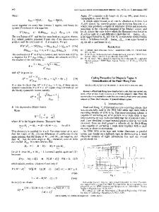
The pusher-puller model of hydrodynamic propulsion has proven useful for studying the behavior of active suspensions.10,11 For instance, flagellates propelled from behind by a rotating helical bundle are “pushers” while those swimming towards the bundle are “pullers.” These are the examples of dipole swimmers, so-called because the disturbance flow generated by the swimmer has the form of that due to a force dipole. Here, we present a version which is indicative of the implicit swimming gait. Consider two spherical particles bound as a rigid assembly (depicted in Fig. 1). On one, denoted 1, we allow for a surface deformation such that

Phys. Fluids 23, 071901 (2011)

E1 ¼ EðI 3ddÞ;

(45)

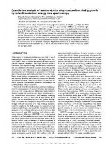
where E is the dipole strength and d is the unit vector connecting the two spheres. All other deformational modes on the particle surfaces are zero. This deformation gives rise to an axisymmetric flow drawing fluid in from the surrounding and streaming it out along d (or the opposite depending on the sign of E). On one side of particle 1, the fluid is free to flow away from the assembly while on the other side it encounters the second particle and is retarded. To conserve mass, a pressure gradient arises along the length of the assembly and propels it away from the free stream (to the right in the figure). With the sign of E reversed, the assembly moves toward the inward streaming fluid. The former is an example of a pusher while the latter is a puller. In fact, these are the purest possible pushing and pulling deformations and thus quite useful as a toy model. For that matter, a quadrupolar swimmer is realized by allowing particle 2 to deform as well with E2 ¼ E1. Here, no net fluid is drawn in from the surroundings, but two streams, one inward and one outward stem from either end of the assembly much like a conveyor drawing the swimmer through the fluid. The aspect ratio of such a body is hardly fixed. A long rod subject to a dipolar deformation is easily realized as a string of N particles, with particles 1–M, M < N, having surface deformations E1, or in general any set of E’s. The set of deformations on all the particles is termed as the implicit swimming gait. In Fig. 2, we plot the swimming speed and rate of energy dissipation of such pushers and pullers as a function of N and M. From Eq. (44), the rate of dissipation due to the swimming is simply (S þ x FC): E. The order of magnitude of E_ is set by the nearest neighbor inter-particle spacing which in this case is R ¼ 2.01 a and scales roughly as (R–2a)1 from hydrodynamic lubrication—the “straining flow,” E1, draws fluid into the gap between nearly touching spheres. Additionally, the longer the swimmer, the slower it goes. Increasing the number of active particles (M) merely produces flows which are stifled by the other nearby particles. Active particles near the end of the rod produce the majority of the thrust so that adding more particles (even if they are active) only increases the drag. A different result may be achieved by structuring the rod-like swimmer as a quadrupole as in Fig. 1. 2. Spinners—The explicit swimming gait

FIG. 1. (Color online) A pusher and a puller (dipoles) and a push-puller (quadrupole) are illustrated. Because the fluid cannot flow freely in the gap between the particles in response to the implicit swimming gait, a pressure gradient forms and drives the swimmer through the fluid.

A spinner may be thought of as the discrete analogue to the swimming torus which invaginates, dragging fluid through its center and around its outside. Fluid struggles to squeeze through the center of the torus generating a pressure gradient that propels the torus in the same direction as the fluid flowing through its center. Our model of the spinner is an example of a swimmer with an explicit swimming gait. Consider the simplest possible spinner formed by two spherical particles, a fixed distance apart and counter rotating about their centers along an axis perpendicular to the line connecting their centers, d. The swimming gait for each particle is ðaÞ

US ðtÞ ¼ Xð0; 0; 0; 6dÞ;

(46)


071901-9


Phys. Fluids 23, 071901 (2011)

FIG. 3. (Color online) The most primitive spinner is built from two spherical particles rolling at fixed separation as though calendaring the fluid between them. In the limit that R ! a, the rate of energy dissipation diverges logarithmically with respect to the separation. This is a consequence of the strong lubrication forces experienced when the gap between the spheres is narrow.

FIG. 2. The swimming speed and rate of energy dissipation of pushers=pullers are plotted. These swimmers are constructed as chains of N particles, the first M of which have the implicit swimming gait E1. The rate of dissipation is so large because the inter-particle spacing is 2.01 a. As such, the nonaffine deformation of neighboring particles induces large stresslets and thus a large rate of dissipation.

where X is the rate of rotation. Interestingly, no constraining force is required to fix the distance between the particles because of symmetry. In the limit that the distance between the particle surfaces, 2(R–a), approaches zero, lubrication arguments can be used to show that the swimming speed is independent of R to first order. While when the particles are widely separated, the swimming speed scales as R2 as the propulsion is driven by the force-rotation coupling. Figure 3 depicts the swimming speed of these two particle spinners as a function of separation. The swimming toroid introduced by Taylor22 and reinvented by Purcell23 may be constructed as a rigid assembly of N particles whose centers lie on the circumference of a circle of radius R so that for particle a, 2pða 1Þ 2pða 1Þ ðaÞ ; R sin ; 0 : (47) x ¼ R cos N N The two particle spinner is merely the case: N ¼ 2. For the swimming gait, we specify that the translational components

of the gait velocity of all the particles are zero. The rotational components of the gait are determined, such that particle a rotates with rate X about the vector tangent to the circle of radius R, i.e., 2pða 1Þ 2pða 1Þ ðaÞ US ¼ X 0; 0; 0; sin ; cos ;0 : N N (48) The surface velocity is constant in time and always normal to the circumferential axis of the toroid. Analytical predictions of the swimming speed and efficiency of such a toroidal swimmer were generated by Leshanksy and Kenneth.24 A good agreement was found between their separation of variables solution to the Stokes equations and the expression put forward by Thaokar et al.25 for swimming toroids with asymptotically large aspect ratios (r=R ! 0). The swimming speed U in this limit is U r 8R 1 log ; Xr 2R r 2

(49)

where r is the minor radius of the toroid. In the case of the simulations, r is the average minor radius of the toroid as the spheres make the toroidal surface bumpy (i.e., r ¼ pa=4). Figure 4 demonstrates the congruence of the exact solutions and the properly normalized simulations. Discrepancies at small ratios of major to minor radius are due to the discrete nature of the models. One way to study toroids in the range of R=r 1 would be to assemble the toroid from particles placed on the surface of a cylinder of radius r and length 2pR which is then wrapped so that the cylinder’s center is co-linear with a circle of radius R. In that case, the ratio of r to R may be arbitrarily close to unity. A modified swimming


071901-10

Swan et al.

Phys. Fluids 23, 071901 (2011)

FIG. 4. (Color online) The toroidal swimmer moves in the same direction as the fluid flowing through its center. When the mean, minor radius of the toroid is used to rescale the swimming speed and aspect ratio, the swimming speed of the rigid assembly and a solid toroid collapse on top of one another. The rate at which fluid is pumped through its center is the most important factor in setting the swimming speed of the toroid. Therefore, the mean, minor radius sets the appropriate velocity scale Xr, the average surface velocity of the rigid assembly.

gait will be needed since the particles in this configuration represent an effectively incompressible surface. B. Purcell’s three-link swimmer

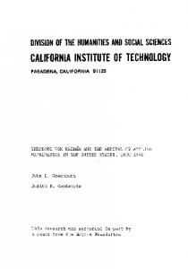
Purcell’s three-link swimmer is an artificial swimmer that illustrates the importance of time-reversal symmetry in Stokes flow.23 A central body has a pair of hinges on either end to which a pair of rudders is attached (see Fig. 5). The angles formed between the rudders and the central body, denoted h1 ðtÞ and h2 ðtÞ, are the only degrees of freedom describing the swimming gait. The gait is characterized by a closed path in time through the angular phase-space. Since the Stokes equations are time-reversible, any trajectory through phase-space that is reciprocal (i.e., the closed path in phase space contains zero area) cannot produce net motion of the swimmer. The swimming gait in which one rudder is held fixed while the other flaps is an example of such a reciprocal path. Clearly, a minimum of two degrees of freedom are necessary to achieve net propulsion at low Reynolds number. In Fig. 5, this reciprocal path, a standard path describing the alternating flapping of each rudder and a complex path are depicted. We construct a three-link swimmer from a rigid assembly of 3 N particles (N particles compose each segment of the swimming body and particles are separated by 2.01 a), and a video of one such swimmer is available online as part of the supplementary material.37 The swimming gait for particle a on rudder i is ðaÞ US ðtÞ ¼ h_i ðtÞðqai sin hi ðtÞ; qai cos hi ðtÞ; 0; 0; 0; 1Þ;

(50)

FIG. 5. (Color online) Purcell’s three-link swimmer is an illustration of the “simplest animal that can swim that way.” At least two degrees of freedom in the parameter space characterizing the configuration of any swimmer are needed in order to achieve net propulsion. Three possible paths through phase space are shown. The reciprocal path gives rise to no net motion while the standard path in which one rudder is held fixed while the other flaps in alternating fashion is the path studied via Stokesian Dynamics. Note, if the three links are all of the same length, then p < h1 ðtÞ þ h2 ðtÞ < p as these configurations prevent the rudders from colliding. The excluded regions of phase space are marked explicitly on the diagram.

where qai is the distance of particle a from its hinge. ðaÞ US ðtÞ ¼ 0 when a corresponds to a particle on the center link. The rudders cycle alternately from hmax to hmax or the converse at uniform rate jh_i ðtÞj ¼ X. It can be shown that the net propulsion is independent of any time dependence of _ the rate hðtÞ, and therefore these swimming gaits are equivalent to those studied by Becker et al.26 for which the “propulsive torque” was held constant [that torque being _ ]. The resulting swimming equivalent to the average of hðtÞ speed over one complete transit of the phase path is plotted in Fig. 6 as a function of hmax . We observe, as did Becker et al., that the swimming velocity increases with hmax until approximately 60 and beyond that the velocity decreases monotonically. We have normalized the swimming speed by the speed of the tip of the rudders multiplied by the resistance couple between torque and rotation for a slender rod. This quantity is similar to the mean torque about each of the hinges. The differences between the simulations and the slender body theory arise from the hydrodynamic interactions among the rudders and the body, something for which


071901-11


Phys. Fluids 23, 071901 (2011)

Becker et al. do not account, as well as the choice of normalization. C. Taylor’s helical swimmer

FIG. 6. (Color online) The swimming speed of Purcell’s three-link swimmer is plotted as a function of the maximum stroke angle, hmax , and the number of particles composing each link, N. The speed is normalized by the tip speed of a rudder as it carries out its stroke. An additional normalization by a factor depending on the logarithm of the length of the rudder, denoted 1 ¼ logðL=2aÞ, which is the couple between rotation and torque for slender bodies. The curve is the swimming speed predicted by Becker et al.26 using slender body theory for rudders moving with a constant torque difference relative to the body.

Sir Geoffrey Taylor directs and narrates one film, Low Reynolds Number Flow, in the series Illustrated Experiments in Fluid Mechanics (1961–1969) by the National Committee for Fluid Mechanics Films. Among the topics discussed is swimming at low Reynolds number, and the physical principles are demonstrated by a novel swimmer composed of two counter-handed, counter-rotating helices (see the original film notes, Fig. 7). We replicate this classic demonstration via Stokesian Dynamics by constructing a rigid assembly composed of particles of radius a whose centers fall on a pair of counterhanded helices with neighboring particles separated by 2.01 a (see Fig. 8). The swimming gait, US(t) is designed so that the particles on each helix rotate about the swimmer’s longitudinal axis with angular velocity 6X. That is, the helices are counter-rotating. In particular, the swimming gait associated with particle a is DrðaÞ d ðaÞ (51) US ðtÞ ¼ X pffiffiffiffiffiffiffiffiffiffiffiffiffiffiffiffiffiffiffiffiffiffiffiffi ; 6d ; DrðaÞ DrðaÞ where DrðaÞ is the vector pointing from the geometric center of the swimmer to the center of particle a and d is the unit

FIG. 7. Taylor’s helical swimmer as depicted in the film Low Reynolds Number Flow. As shown in the film, the fish-like swimmer (middle of the figure) cannot swim in high viscosity fluids because of time-reversal symmetry.


071901-12

Swan et al.

Phys. Fluids 23, 071901 (2011)

FIG. 9. (Color online) The velocities of helical swimmers satisfying the slender-body and long wavelength conditions (L > 2p=k > R > a) are normalized by the velocity of Taylor’s swimming sheet and plotted as a function of the ratio of swimmer length to helical arc length, denoted s. This results in a collapse of the data onto a universal curve that the slender-body theory matches in functional form over a wide range of s.

FIG. 8. (Color online) Taylor’s helical swimmer is constructed from spherical particles of radius a. The top helix has a clockwise orientation (righthanded as depicted) while the bottom helix has a counter-clockwise orientation. The spherical particles are colored in quadrants to aid visualization of the relative orientations.

vector parallel to the long axis of the swimmer. We measure the resultant swimming velocity, denoted U, as a function of the number of particles composing the entire body, N; the helix radius, R; and the helical wavelength, 2p=k. The end to end length of the swimmer, denoted L, may be computed as a function of these parameters. Notice that when the helix is projected onto a twodimensional space it takes the form of a traveling wave. In fact, G.I. Taylor studied this, the so-called swimming sheet problem, extensively.27 In the two-dimensional domain, a point on the surface of the swimming sheet has velocity normal to the swimming direction, kR sinðkx XtÞ, and velocity, U, along the swimming direction. The swimming speed is determined by necessitating that the hydrodynamic force on the sheet is zero (there is no restriction on the torque in two dimensions). In the limit that the traveling wave has a small amplitude and a large wavelength (kR 1), the swimming speed is kR2 X=2. As the counter-rotating helices are essentially the three-dimensional analogue of the swimming

sheet, we normalize the swimming speed of the helical swimmer by this same factor. We expect that this same scaling yields a universal curve for predicting the swimming speed of the helical swimmer. Figure 9 depicts the results of Stokesian Dynamics simulations of Taylor’s helical swimmer. A variety of parameter choices are employed in the study, though they all conform to the dimensional hierarchy: L > 2p=k > R > a, such that these helices approximate the small amplitude, long-wavelength limit. The particular values are given in Table I for which all combinations were tested. A video of one of Taylor’s helical swimmers is available as a part of the supplementary material online. When plotted as a function of the swimmer length (not shown), we observe that the data center around several distinct curves in which every data point corresponds to swimmers composed of the same number of particles. Rescaling the length of the swimmers on the number of particles composing the swimmer s ¼ L=(2 a N) produces a TABLE I. The number of particles, helical wave number, and helical wavelength studied for Taylor’s swimming helices. All combinations of these variables were employed. N

ka

R=a

100 200 300 400

0.096 0.140 0.180 0.251 0.419 0.628

4 5 6 7


071901-13


Phys. Fluids 23, 071901 (2011)

universal curve. This quantity is the ratio of the length of the swimmer to arc length of the helices and has a well known form in terms of the helix wave number and radius, qffiffiffiffiffiffiffiffiffiffiffiffiffiffiffiffiffiffiffi 1= 1 þ ðkRÞ2 . The collapse of data across such a variety of parameters suggests that this ratio has physical as well as geometric significance. Namely, the drag on a body at low Reynolds number is typically proportional to its largest dimension (in this case, L). The propulsive thrust is also proportional to the swimmer’s extent, but depends to first order on the area available for propulsion as well. Therefore, helical swimmers can be expected to behave similarly when the ratio of the length to arc length is comparable. A resistive force theory prediction in the long-wavelength limit suggests that this curve should have the form 2 s2=(s2–2).28 Surprisingly, the resistive force theory (which should only be valid in the limit that s ! 1) fits the data over almost the entire range of s. Though, we have not studied helical swimmers for which the wavelength is longer than the body or the radius is larger than the wavelength, etc. These may not have the same physical behavior. Notice how a simple simulation can not only confirm a relatively complicated resistive force theory analysis but can also bound its applicability. It is impossible to decide the explicit range of applicability of an asymptotic analysis without comparison with experiment or simulation.

versely, the constant volume condition restricts the functional form of sðh; /; tÞ. A two-dimensional amoeboid for which conformal mapping techniques allow for analytical solution of the Stokes equations has the shape29 ZðtÞ sðh; tÞ ¼ R ðWðtÞ YðtÞÞ sin h pffiffiffi sin 2h; 2 ZðtÞ ðWðtÞ þ YðtÞÞ cos h þ pffiffiffi cos 2h þ XðtÞ ; (53) 2 where R sets the length scale for the swimmer, and W(t), X(t), Y(t), and Z(t) are phase space parameters describing the time dependence of the swimming gait. Because the swimmer is two-dimensional, it is characterized by a single parameter h 2 ½0; 2pÞ. The condition of constant volume (or area in this case which we choose to fix as pR2 ) specifies W(t) such that WðtÞ2 ¼ YðtÞ2 þ ZðtÞ2 þ 1;

while the condition of immobile center of mass constrains X(t). Certain combinations of the phase space variables can result in swimmer shapes for which the contour of the swimmer overlaps itself. Self-interaction may be precluded from the set of all possible swimmers by two conditions pffiffiffi WðtÞ YðtÞ6 2ZðtÞ;

(55)

WðtÞYðtÞ 2ZðtÞ2 WðtÞ2 :

(56)

D. Amoeba-like swimming

Amoebas comprise a class of so-called large deformation swimmers. Unlike that of flagellates for which the variation in tail shape is often small when compared to the extent of the swimmer and ciliates for which the deformation occurs in a small envelope surrounding the swimmer, amoebas undergo deformations on the same scale as the body itself. The same hydrodynamic principles apply, though the analysis of such swimmers is limited by the solvability of the Stokes equations for bodies with a variety of complex geometries. Three key constraints are necessary to adapt Stokesian Dynamics to modeling amoebas: the swimming gait must conserve the volume of the swimmer, the swimming gait must be inextensible and the swimming gait must introduce no variation in the swimmer’s geometric center. The first two are practical restrictions that prevent the particles comprising the surface of the swimmer from colliding. The latter constraint forces the swimming gait to coincide with the definition employed throughout this manuscript. The shape of the swimmer is defined as a function of time, and points on the swimmer’s surface are denoted sðh; /; tÞ where the variables h and / parameterize the surface. The swimming gait is then uS ðtÞ ¼ s_ ðh; /; tÞ þ uh ðh; /; tÞth þ u/ ðh; /; tÞt/ ;

(52)

where th and t/ are two mutually orthogonal vectors tangent to the surface. The tangential components of the velocity may be chosen freely. We use them to enforce the condition that particles remain uniformly distributed over the swimmer’s surface. The result is that there is no relative, tangential velocity among nearby points on the surface. Con-

(54)

With these conditions, we can view the phase space of the amoeboid swimmer in just two dimensions. Figure 10 depicts the phase space in Y(t) and Z(t) as well as paths through that space. In particular, we study the net propulsive speed of this class of amoeboid with phase space variables satisfying YðtÞ ¼ r cosðxtÞ, ZðtÞ ¼ r sinðxtÞ. The frequency of the phase space orbit is denoted x while the radius of the orbit is denoted r. This amoeboid may be constructed from N particles, where N and the scale of the swimmer R are related in a complex manner such that exactly N evenly spaced particles line the swimmer’s contour. Since the initial swimmer shape (t ¼ isffi elliptical with major and minor axes p0) ffiffiffiffiffiffiffiffiffiffiffiffi Rð 1 þ r2 6rÞ, respectively, the particles are distributed so that: jxðaþ1Þ xðaÞ j2 ¼ d2

(57)

and ðaÞ

x1 pffiffiffiffiffiffiffiffiffiffiffiffi ffi 1 þ r2 þ r

!2

ðaÞ

x2 ffi þ pffiffiffiffiffiffiffiffiffiffiffiffi 1 þ r2 r

!2 ¼ R2 :

(58)

We have chosen the inter-particle spacing d ¼ 2.01 a. A particle a is subject to the swimming gait, ðaÞ

ðaÞ ðaÞ

US ¼ s_ ðhðaÞ ; tÞ þ uh th ;

(59)


071901-14

Swan et al.

Phys. Fluids 23, 071901 (2011)

FIG. 11. The swimming speed of amoebas subject to a circular phase space orbit with radius r is compared for swimmers composed of 32, 52, 100, and 152 particles. The number of particles, N, was chosen as a multiple of four for symmetry purposes. The speed of two-dimensional amoebas is also depicted. It is smaller than that of the monolayer swimmers because fluid may flow freely above, below, and through the swimmers composed of spherical particles.

FIG. 10. (Color online) The shape of the amoeboid is constrained by conditions of constant volume and no self-interaction. The valid phase space in variables Y(t) and Z(t) is depicted as well as the circular phase space orbits studied herein. The shape of a particular amoeba is shown evolving in time (steps 1–8) with increased thickness and decreased opacity both corresponding to longer times. This amoeba arises from a circular phase space orbit with r ¼ 0.5.

where hðaÞ denotes the parametric position of particle a and ðaÞ ðaÞ uh th is the velocity of particle a tangential to the swimmer’s contour. The tangential velocity is determined by restricting the relative tangential motion of all the neighboring particles to a uniform rate Q such that ðaþ1Þ

ðUS

ðaÞ

US Þ Drðaþ1;aÞ ¼ Q;

(60)

where Drðaþ1;aÞ is the unit vector pointing along the line connecting the centers of particles a and a þ 1. The rate, Q, as well as the tangential components of the velocity field are found by solving Eq. (60) simultaneously for all neighboring particle pairs (a ¼ 1:::N). This is sufficient to keep the particles from overlapping because of the prescribed stroke and is equivalent to a condition limiting the swimmer’s extensibility. Figure 11 details the average rate of propulsion (U) of the amoeba-like swimmer as a function of the size of the phase space orbit. Larger values of r correspond to more eccentric swimming strokes. The example depicted in Fig. 10 is at the limits of the constrained phase space and a video of this swimmer built from spherical particles is available

online as supplementary material.37 It is as eccentric as the prescribed conditions of constant volume and no self-interaction allow. Following the work of Avron et al.,30 which uses conformal mapping techniques to solve the Stokes equations, we find a simple closed form prediction for the mean speed of the amoeboid subject to the circular path through [Y(t), Z(t)] phase space, viz. pffiffiffi ð 2 U 1 2p=X ZðtÞ _ r2 pffiffiffiffiffiffiffiffiffiffiffiffiffi : (61) pffiffiffi ¼ YðtÞdt ¼ 4 xR 2p 0 2WðtÞ 1 þ r2 Indeed, our simulations recover the scaling expected from this two-dimensional analysis with respect to the eccentricity of the stroke. The difference in leading coefficient is attributable to the fact that the simulated swimmer is a monolayer in an otherwise fully three-dimensional fluid domain, while the analytical analysis applies to a strictly two-dimensional swimmer. That fluid may flow above, below, and through our simulated amoeboid certainly affects the propulsive rate, though apparently not its functional dependence on the swimming stroke. VIII. EXTENSIONS

We have detailed the classical formulation for hydrodynamic self-propulsion at low Reynolds number and its direct analogue in the mechanics of particles in low-Reynolds-number flows. Validation of this analogy was demonstrated by the study of several swimming problems: pushers and pullers, spinners, Purcell’s three-link swimmer, and Taylor’s counter rotating helices, while the flexibility of such a method was illustrated with simulations of an amoeboid. These examples


071901-15


Phys. Fluids 23, 071901 (2011)

constitute only a fraction of possible constructions. In fact, we have omitted several interesting circumstances for which the Stokesian Dynamics method of swimming is ideally suited. The preceding discussion often took for granted that the Stokesian Dynamics formulation for swimming is not restricted to the kinematics of a single body. Rather, the number of selfpropelled bodies is arbitrary and requires no change in the method as depicted. Throughout we have studied swimmers with prescribed swimming kinematics. In particular, the rate of deformation of the swimming body is fixed via the swimming gait US(t). Alternatively, the rate at which the body dissipates energy, _ EðtÞ, may be held constant such that the body swims with constant power. The rate of energy dissipation is quadratic in US(t) such that _ US ðtÞ US ðtÞ; EðtÞ

(62)

^ is proportional to the while the swimming speed itself, U, swimming gait. Thus, the constant power swimming speed, ~ is U, ^ 1 U ðtÞ ~ ¼ qU ffiffiffiffiffiffiffiffiffi ¼ R RFU RT R RFU qSffiffiffiffiffiffiffiffiffi ; U _ _ EðtÞ EðtÞ

FIG. 12. (Color online) A flexible oar is constructed by connecting many rigid assemblies (dumb-bells) with linear springs. The swimming gait emerges through articulation of the springs by changing their rest length.

(63)

qffiffiffiffiffiffiffiffiffi _ is the effective swimming gait. and the ratio US ðtÞ= EðtÞ Obviously, the average speed of such swimmers is different from those propelled by fixed rate of deformation as the effective swimming rate now has a complicated dependence on time and the configuration of the assemblage of particles _ via EðtÞ. However, nothing in the Stokesian Dynamics method precludes the study of such constant power bodies. Similarly, rather than fixing the kinematics, it is possible to control the swimming stroke dynamically through knowledge of the local stress state of the swimmer. It has been observed that cooperative beating of flagella requires some degree of kinematic response.8 In this case it is the internal stresses of the flagellum that dictate how it will move next. Again, these stresses are known in the context of Stokesian Dynamics simulations as the stresslets on each of the particles. We foresee at least two ways in which reactive kinematics may be implemented. First, a particular stress state may be specified and then the driving swimming gait computed. This requires the inversion of RSE to determine US(t) and is analogous to the constant power kinematics just described. Here, however, the rate of dissipation due to each particle is fixed rather than the rate of dissipation for the whole swimmer. Second, a control scheme may be implemented such that the swimming gait at time t depends in some fashion on the internal stresses at past times. Just as Stokesian Dynamics makes it possible to detail the dynamics of particles without explicitly solving for the fluid velocity field everywhere in space, it also facilitates the computation of a swimmer’s internal stresses without requiring specification or solution of a model for the body’s internal mechanics. In lieu of a specified relationship between the internal stress state of the swimmer and the swimming gait, a swimmer may be fashioned as a set of rigid bodies and

springs and articulated by changing the rest length of the springs. We illustrate a flexible oar-type swimmer in Fig. 12. Here, a set of rigid dumb-bells constructed from pairs of spherical particles (see Sec. V) is arranged linearly (normal to the dumb-bell axis) and neighboring pairs of spheres connected with linear springs. On the left side of the swimmer, the springs have rest length L1(t) and on the right side the springs have rest length L2(t). By varying the rest lengths in time (these constituting the minimum two degrees of freedom required for net propulsion at low Reynolds number),23 the arrangement of dumb-bells can be made to arch flexibly to and fro. It swims in a snake-like manner. The forces the springs exert on the beads take the form of inter-particle forces which we have denoted FP throughout the article. Since the inter-particle forces are mutual (Newton’s first law), they exert no net force on the swimmer just as the constraining forces. In this way, the swimming gait emerges through active manipulation of the internal stresses of the swimmer. We perform a sample calculation for the swimmer in Fig. 12 subject to a traveling wave articulation. That is, the rest lengths of the springs [L1(t), L2(t)] switch from (2 a, 3 a) to (3 a, 2 a), one after another down the length of the swimmer. The time between the switching of one spring and the next is x1 , and the intra-dumb-bell spacing is 2.01 a. Figure 13 shows an inverse relationship between switching frequency and swimmer speed. Here, however, the swimming is as a result of imposing the internal stresses and no implicit or explicit swimming gait is needed. To be sure, the choice of model for these stresses has some impact on the resulting swimming motion because, in addition to controlling the rate at which the swimmer changes shape, these stresses control what shapes the swimmer can take throughout the gait. But note that the body shape is


071901-16

Swan et al.

FIG. 13. (Color online) The swimming speed of a flexible oar is decays with increasing frequency of articulation. The swimming results from a traveling wave-type articulation of the spring rest lengths forming the connection among the swimmer’s constituent dumb-bells. The spring constant is denoted k and serves as a factor for normalization.

determined by both the actuating stresses and the hydrodynamic interactions between different parts of the body. An approach such as this is one way of testing various mechanisms (for there are surely more than the Hookian spring model) and determining which are and which are not suitable for efficient swimming of particular bodies. The resistance tensors encompass the entire dependence of the propulsive speed on the swimmer geometry (i.e., the relative positions of the particles comprising a swimmer). This statement is even more general as the resistance tensor also encompasses the hydrodynamic interactions among the particles and any confining geometry. Therefore, the same methodology may be applied to model swimmers near macroscopic surfaces such as a solid wall, a fluid-fluid interface, the inside of channels or tubes, etc. without modification. To do so, however, the “correct” resistance tensors are needed. For instance, Stokesian Dynamics has been used to construct the resistance tensors for particles near a single wall19 or in a channel,20 and these can be employed directly in the formulation here. Extensions to more exotic cases require some detailed analysis regarding the hydrodynamics of a single particle in that specific geometry. Though in principle, there are no restrictions on the present formulation of the swimming problem. Of course active suspensions—that is, suspensions of self-propelled bodies—may be modeled through exactly the same means. As is common in computational simulations, a suspension of particles or swimmers, must be treated as a system of periodically replicated unit cells filled with fluid and swimmers. By analogy with swimming in confined geometries, the periodic boundary condition on the each edge of the simulation cell may be regarded as that due to a macroscopic boundary. In principle it is no different from

Phys. Fluids 23, 071901 (2011)

the no-slip condition on a rigid, impenetrable wall. As such, no modification to the formulation of the swimming problem using rigid assemblies of particles is needed. Rather, the appropriate resistance tensor for a periodic system, something which is well known,18 must be employed. Our method for simulating swimmers allows for the choice of modeling the swimming kinematics either implicitly or explicitly [Eqs. (39) and (41), respectively]. The former allows for facile modeling of the long range hydrodynamic interactions among swimmers. This neglects the details of the propulsive mechanism and therefore the precise near-field interactions. The latter, on the other hand, captures both of these effects at the cost of requiring more particles to model the same number of swimmers. Active suspensions may be modeled at many different levels in this fashion. It may even be possible to implement a multi-level modeling scheme which allows for inclusion of the near-field details with implicit kinematics by performing parallel computations on swimmers with explicit kinematics. Note too that there is no restriction on the identity of the rigid bodies employed in this formulation. As such, it is possible to generate a system with a single swimmer surrounded by many singleton particles which could be Brownian. This is an ideal model for swimming in non-Newtonian fluids. Recent research efforts have focused on just this by treating the non-Newtonian fluid as a continuum.31 As the Brownian time scale is proportional to the cube of the size of the diffusing object, this same limit is achieved by swimmers perhaps as little as three times larger than the surrounding particles. However, this method is hardly restricted to the continuum limit and systems in which the swimmer is the same size as (or smaller than) the passive particles may be modeled too. In order to incorporate Brownian motion, the Brownian forces on the particles and swimmer must be determined in terms of the constrained resistance tensor R RFU RT rather than the resistance tensor itself. The instantaneous mean square Brownian force, F B, on the particles and swimmer is R FB FB RT ¼ 2kTR RFU RT ;

(64)

where kT is the thermal energy. It may not always be possible to determine the resistance tensor in a form amenable for such computations. In such a case, a Langrange multiplier approach may be employed instead.32 Finally, we have made available as supplemental material to this article, an open source version of our Stokesian Dynamics code designed to model a single hydrodynamically self-propelled body. Both the implicit and explicit swimming gaits may be modeled with this code. Note though, the force=velocity moments are computed up to the couplet=gradient (dipole) levels. As such, simulation of spherical quadrupolar squirmers5,21 requires additional code for computing all the quadrupolar elements of the force and velocity moments in the context of the Stokesian Dynamics method. The relevant hydrodynamic functions are known, however.34,35 Alternatively, one could construct a “sphereof-spheres” with the appropriate implicit gait on the constituent spheres. There are natural examples of such spherical


071901-17


Phys. Fluids 23, 071901 (2011)

colonies such as Volvox barberi and Volvox carteri.36 Determination of these higher order moments or the appropriate sphere-of-spheres implicit gait is left to the motivated reader. The code is free to use or adapt, though acknowledgement of the copyright holders must be made and this manuscript cited in any published work. It is hoped that by using this code the burden of the hydrodynamics of low-Reynolds-number swimming may be removed and more attention and energy given to the important biophysical questions of swimming microorganisms. The code may also prove useful in the design of artificial swimmers both de novo and de natura. ACKNOWLEDGMENTS

The motivation for this work arose from a special topics course, ChE 174, on self-propulsion at low Reynolds number given in the spring of 2010 at the California Institute of Technology—hence the title “Teaching Stokesian Dynamics to swim.” Participants were Lawrence Dooling (pushers and pullers), Nicholas Hoh (pushers and pullers), Jonathan Choi (spinners) and Roseanna Zia (toroids). We thank them for their contributions to the course and this work. This work was supported in part by NSF Grant Nos. CBET 0506701 and CBET 074967.

faster. Additional physical insight may be drawn from this approach, so it is useful to depict it in detail. For these purposes, one additional notation change is needed. The quantity R2B;exact R2B;1 is denoted Rnf such that the resistance tensors contained therein are denoted Rnf FU for example. The superscript nf stands for “near-field” as the exact near-field hydrodynamic interactions are embedded in this quantity. Note, we have again chosen to truncate the far-field mobility at the stresslet level. Consider that the hydrodynamic forces on particles in low-Reynolds-number flows (though this may be true in finite-Reynolds-number flows as well) are a superposition of those arising from lubrication (denoted Fnf as they come from fluid mediated interactions among nearly touching particles) and those arising from the many-bodied hydrodynamic interactions (denoted Fff). Without loss of generality, the near-field forces may be written as nf Fnf ¼ Rnf FU U RFE : E:

Then Newton’s second law in the absence of inertia [Eq. (25)] becomes nf ff P 0 ¼ Rnf FU U þ F RFE : E þ F ;

APPENDIX A: ITERATIVE SOLUTION FOR THE HYDRODYNAMIC FORCE, TORQUE, AND STRESSLET

It is frequently the case that the system of particles under consideration is large such that O(N3) calculations requires a prohibitive amount of computational time. Another formulation of the Stokesian Dynamics procedure avoids the explicit inversion of the mobility and resistance tensors. Instead, the iterative inversion of these quantities is employed reducing the computational scaling to O(N2) or

~ ff F Sff

!

" ¼ M þ " kM1

and U¼

1 ~ ff ~ nf F R FU

Rnf FE

~ Þ1 ðR FU 0

:EþF

P

;

0 0

(A2)

where the far-field forces are defined self-consistently by solution of ff U F 1 ; (A3) ¼ M E Sff where Sff is the far-field contribution to the hydrodynamic stresslet. With a few algebraic manipulations, this system of equations can be solved for the far-field hydrodynamic force and the particle velocities as

!#1 ~ nf Þ1 0 ðR FU kM 0 0 ! !# nf 1 nf ~ Þ ðFP Rnf : EÞ ~ Þ1 ðFP Rnf : EÞ ðR ð R FE FE FU FU ; 0 E nf

1

(A1)

!

1

(A5)

~ nf ¼ Rnf þ kI, I is the where k is an arbitrary coefficient, R FU FU ff ~ ¼ Fff þ kU. Since Rnf by itself is not idem tensor, and F FU always invertible, an additional diagonal tensor is added to make it positive definite. A value of 6pga for k will always ~ nf invertible and naturally recovers the suffice to make R FU exact solution for the sedimentation rate of a single particle with radius a. Notice, that the near-field hydrodynamic interactions dominate the hydrodynamic force. In fact, Eq. (A5) may be interpreted as the definition of the particles’ rigid body

(A4)

motion in terms of the near-field contributions to the resistance tensor only. The far-field hydrodynamic force simply assumes whatever value is self-consistent with that rigid body motion. The condition of self-consistency is given by Eq. (A3). It can be demonstrated with little effort that this prescription is identical to the list of approximations, inversions, and the final summation previously described. The difference, however, is that the far-field mobility tensor (typically a dense algebraic structure) is never inverted explicitly. Rather, the sum of the far-field mobility and the inverse of Rnf FU (a sparse matrix) are inverted in the computation of the far-field hydrodynamic forces. This distinction is important because the iterative inversion of Rnf FU may be


071901-18

Swan et al.

Phys. Fluids 23, 071901 (2011)

accomplished with O(N) computations. The far-field forces may also be computed iteratively with only the product of the bracketed and inverted tensor in Eq. (A4) and an arbitrary vector being required. Consequently, the product of M1 and an arbitrary vector are needed. The explicit calculation of M1 itself requires at most O(N2) computations; therefore, this approach to Stokesian Dynamics requires at most O(N2) computations in calculating the hydrodynamic forces on and the velocities of N particles. The computational scaling depends on how quickly the product of M1 and a vector can be formulated. Schemes such as Accelerated Stokesian Dynamics use the fast Fourier transformation to accomplish this in OðN log NÞ calculations.18 Though this only applies to infinite and periodic suspensions and not to

finite collections of particles. In principle, the fast multipole method can be employed to compute the product of M1 and any vector in O(N) computations regardless of whether the system consists of a finite number of particles or is a suspension. APPENDIX B: ITERATIVE SOLUTION FOR THE CONSTRAINED HYDRODYNAMIC FORCE, TORQUE, AND STRESSLET

Following the previous appendix, the far-field forces on the particles comprising rigid assemblies and velocities of the rigid assemblies themselves are defined as the solution to,

0 1 1 nf nf T P ~ I 0 R F RFE : E A R RFU R @ I kM1 0 0 E 8 0 19 1 nf = < T T ~ I 0 R 0 A R R RFU R ¼ M1 þ kM1 @ : 0 0 0 0 ;

and 1 ff ~ Rnf : E þ FP ; ^ ¼ RR ~ NF RT R F U FE FU

(B2)

~ ff remain the ~ nf and F respectively. The definitions of R FU same. One more brief note regarding computation is necessary here. As R is block diagonal, it is also sparse. Therefore, sparse matrix methods may be applied to it. In particular, the ~ nf RT is sparse and may be computed using quantity R R FU O(N) operations. Therefore, as in Stokesian Dynamics for unconstrained particles, the bottleneck for the algorithm is the determination and inversion of the far-field mobility. Using this iterative prescription for the hydrodynamics of rigid bodies results in the same computational scaling, where there are no constraints at all [i.e., if the algorithm for free particles was OðN log NÞ as with Accelerated Stokesian Dynamics, the algorithm for constrained particles is also OðN log NÞ ]. In fact, because the “effective” near-field resistance, ~ nf RT , for the rigid assemblies is smaller in dimension RR FU ~ nf ; the computation than that for the particles themselves, R FU of the particle velocities and hydrodynamic forces is faster when the particles are constrained. This is in contrast to the experience of Meng and Higdon33 who solved simultaneously for the far-field forces and rigid body velocities and found that the number of iterations required for inversion was on the order of hundreds for even a modest number of particles comprising the system. In the approach just described, we solve for the far-field forces first and then compute the rigid body velocities. The number of iterations required to solve Eq. (B1) is typically no more than 10 to 15 even when thousands of particles are employed. Similarly,

! ~H F FF ; SH FF

(B1)

~ nf RT can be inverted iteratively through the quantity R R FU the use of the incomplete Cholesky preconditioner in only five to ten iterations given a similar number of particles. The numbers of iterations correspond to a typical relative error tolerance of 104. 1

W. B. Whitman, D. C. Coleman, and W. J. Wiebe, “Prokaryotes: The unseen majority,” Proc. Natl. Acad. Sci. 95, 6578, (1998). 2 G. K. Batchelor, An Introduction to Fluid Dynamics (Cambridge University Press, Cambridge, UK, 1967). 3 R. S. K. Barnes, P. P. Calow, P. J. W. Olive, D. W. Golding, and J. I. Spicer, The Invertebrates: A Synthesis, 3rd ed. (Wiley-Blackwell, Malden, MA, 2001). 4 E. E. Keaveny and M. R. Maxey, “Spiral swimming of an artificial microswimmer,” J. Fluid Mech. 598, 293 (2008). 5 T. Ishikawa, M. P. Simmonds, and T. J. Pedley, “Hydrodynamic interaction of two swimming model microorganisms,” J. Fluid Mech. 568, 119 (2006). 6 T. Ishikawa, G. Sekiya, Y. Imai, and T. Yamaguchi, “Hydrodynamic interactions between two swimming bacteria,” Biophys. J. 93, 2217 (2007). 7 A. Kanevsky, M. J. Shelley, and A. Tornberg, “Modeling simple locomotors in Stokes flow,” J. Comp. Phys. 229, 958 (2010). 8 E. Lauga and T. R. Powers, “The hydrodynamics of swimming microorganisms,” Rep. Prog. Phys. 72, 096601 (2009). 9 D. Saintillan and M. Shelley, “Orientational order and instabilities in suspensions of self-locomoting rods,” Phys. Rev. Lett. 99, 058102 (2007). 10 J. P. Hernandez-Ortiz, C. G. Stoltz, and M. D. Graham, “Transport and collective dynamics in suspensions of confined swimming particles,” Phys. Rev. Lett. 95(20), 204501 (2005). 11 P. Underhill, J. P. Hernanadez-Ortiz, and M. D. Graham, “Diffusion and spatial correlations in suspensions of swimming particles,” Phys. Rev. Lett. 100(24), 248101 (2008). 12 S. Kim and S. J. Karrila, Microhydrodynamics, 2nd ed. (Dover Inc., Mineola, NY, 1991). 13 J. F. Brady and G. Bossis, “Stokesian Dynamics,” Ann. Rev. Fluid Mech. 20(1), 111 (1988). 14 H. A. Stone and A. D. T. Samuel, “Propulsion of microorganisms by surface distortions,” Phys. Rev. Lett. 77, 4102 (1996). 15 J. Happel and H. Brenner, Low Reynolds Number Hydrodynamics (Springer, New York, 1983).


071901-19 16


O. A. Ladyzhenskaya, The Mathematical Theory of Viscous Incompressible Flow (Gordon and Breach, New York 1963). 17 L. J. Durlofsky, J. F. Brady, and G. Bossis, “Dynamic simulation of hydrodynamically interacting particles,” J. Fluid Mech. 180, 21 (1987). 18 A. Seirou and J. F. Brady, “Accelerated Stokesian Dynamics,” J. Fluid Mech. 448, 115 (2001). 19 J. W. Swan and J. F. Brady, “Simulation of hydrodynamically interacting particles near a no-slip boundary,” Phys. Fluids 19, 113306 (2007). 20 J. W. Swan and J. F. Brady, “Particle motion between parallel walls: Hydrodynamics and simulation,” Phys. Fluids 22, 103301 (2010). 21 J. R. Blake, “A spherical envelope approach to ciliary propulsion,” J. Fluid Mech. 46, 199 (1971). 22 G. I. Taylor, “The action of waving cylindrical tails in propelling microscopic organisms,” Proc. R. Soc. London Ser. A 211, 225 (1952). 23 E. M. Purcell, “Life at low Reynolds number,” Am. J. Phys. 45(3), 11 (1977). 24 A. M. Leshansky and O. Kenneth, “Surface tank tredding: Propulsion of Purcell’s toroidal swimmer,” Phys. Fluids 20, 063104 (2008). 25 R. M. Thaokar, H. Schiessel, and I. M. Kulıć, “Hydrodynamics of a rotating torus,” Euro. Phys. J. B 60, 325 (2007). 26 L. E. Becker, S. A. Koehler, and H. A. Stone, “On self-propulsion of micro-machines at low Reynolds number: Purcell’s three-link swimmer,” J. Fluid Mech. 490, 15 (2003). 27 G. I. Taylor, “Analysis of the swimming of microscopic organisms,” Proc. R. Soc. London Ser. A 209, 447 (1951).

Phys. Fluids 23, 071901 (2011) 28

E. Lauga, W. R. DiLuzio, G. M. Whitesides, and H. A. Stone, “Swimming in circles: Motion of bacteria near solid boundaries,” Biophys. J. 90, 400 (2006). 29 A. Shapere and F. Wiczek, “Geometry of self-propulsion at low Reynolds number,” J. Fluid Mech. 198, 557 (1989). 30 J. Avron, O. Gat, and O. Kenneth, “Optimal swimming at low Reynolds numbers,” Phys. Rev. Lett. 93(18), 186001 (2004). 31 E. Lauga, “Propulsion in a viscoelastic fluid,” Phys. Fluids 19, 083104 (2007). 32 E. J. Hinch, “Brownian motion with stiff bonds and rigid constraints,” J. Fluid Mech. 271, 219 (1994). 33 Q. Meng and J. J. L. Higdon, “Large scale dynamic simulation of platelike particle suspensions. I. Non-Brownian simulation,” J. Rheology. 51, 1 (2008). 34 A. Nadim and H. A. Stone, “The motion of small particles and droplets in quadratic flows,” Stud. Appl. Math. 85, 53 (1991). 35 S. Haber and H. Brenner, “Hydrodynamic interactions of spherical particles in quadratic Stokes flows,” Int. J. Multi. Flow. 25(6–7), 1009 (1999). 36 K. Drescher, K. C. Leptos, I. Tuval, T. Ishikawa, T. J. Pedley, and R. E. Goldstein, “Dancing Volvox: Hydrodynamic bound stats of swimming algae,” Phys. Rev. Lett. 102, 168101 (2009). 37 See supplementary material at http://dx.doi.org/10.1063/1.3594790 for Stokesian Dynamics source code for use in modeling a single lowReynolds-number swimmer, and movies corresponding to simulations of the helical, three-link, and amoeboid swimmers.


Modeling hydrodynamic self-propulsion with ... - Caltech Authors

Modeling hydrodynamic self-propulsion with ... - Caltech Authors

Suggest Documents

Variability with Wise - Caltech Authors

COMPLEX NUMERICAL MODELING OF ... - Caltech Authors

Shock and detonation modeling with the Mie ... - CalTech Authors

A Suspended Microchannel With Integrated ... - CalTech Authors

Computational experiments with a three ... - Caltech Authors

scillation with Photorefractive Gain - Caltech Authors

Meshkov instability with reshock - Caltech Authors

Progress on Pricing with Peering - Caltech Authors

Mechanical Systems with Symmetry, Variational ... - Caltech Authors

DECIGO Pathfinder - CalTech Authors

Astronomy Astrophysics - CalTech Authors

Gas Streams - Caltech Authors

iiiiiiiiiiiiiiii'iiiiiiiiiiiiiiiii - CalTech Authors

imece2007-43156 - CalTech Authors

physical review - Caltech Authors

Dynamic UNITY - CalTech Authors

WormBase 2007 - CalTech Authors

Supplemental Information_3_6_10_2 - CalTech Authors

Transfection - Caltech Authors

Combustion - Caltech Authors

Q=( d ) - Caltech Authors

Untitled - Caltech Authors

Untitled - Caltech Authors

Transactions Letters - Caltech Authors