Georgia Institute of Technology, School of Aerospace Engineering. Atlanta GA, USA. ... âMechanics Research Communications, 28, pp 571 â 599, 2001. 1 ...
Modeling of Unilateral Contact Conditions with Application to Aerospace Systems Involving Backlash, Freeplay and Friction ∗ Olivier A. Bauchau and Jesus Rodriguez Georgia Institute of Technology, School of Aerospace Engineering Atlanta GA, USA. Carlo L. Bottasso Dipartimento di Ingegneria Aerospaziale, Politecnico di Milano Milano, Italy.
Abstract This paper describes an analysis procedure for the modeling of backlash, freeplay and friction in flexible multibody systems. The first two effects are formulated in a general manner as unilateral contact conditions in multibody dynamics. The incorporation of the effects of friction in joint elements is also discussed, together with an effective computational strategy. These non-standard effects are formulated within the framework of finite element based multibody dynamics that allows the analysis of complex, flexible systems of arbitrary topology. The versatility and generality of the approach are demonstrated by presenting applications to aerospace systems: the flutter analysis of a wing-aileron system with freeplay, the impact of an articulated rotor blade on its droop stop during engagement operation in high wind conditions, and the dynamic response of a space antenna featuring joints with friction.
1
Introduction
Finite element based multibody dynamics formulations extend the applicability of classical finite element methods to the modeling of flexible mechanisms. Such numerical procedures implement a number of generalized elements, each providing a basic functional modeling capability. A general computer code will include rigid and flexible bodies, such as beams and shells, various kinds of joints, and active elements including motors and actuators. Assembling the various elements, it is then possible to construct a virtual prototype of the flexible mechanism with the required level of accuracy. These procedures are designed to overcome the modeling limitations of conventional multibody formulations that are often restricted to the analysis of rigid systems or use a modal representations of the flexibility of ∗
Mechanics Research Communications, 28, pp 571 – 599, 2001.
1
the various parts of the system. Using these new analysis tools, low cost parametric studies of complex systems can be quickly conducted to identify the key variables governing the phenomenon being investigated. Multibody dynamics formulations provide a general and flexible paradigm for the modeling of aerospace systems, and are already playing a crucial role in the design process. Some of the most complex applications of this technology come from the world of rotary wing vehicles. Finite element multibody procedures are now being applied to the comprehensive aeromechanical simulation of helicopters and tilt-rotors, allowing the detailed modeling of such complex components as gimbal mounts, swash plates, bearingless root retention beams, and variable geometry rotors, among many others [1]. Indeed, rotorcraft systems present some of the most challenging applications, because they involve complex topologies, require geometrically exact nonlinear beam elements, and present widely different solution scales that render the governing equations highly stiff. Consequently, multibody formulations that initially dealt with rigid systems presenting simple tree topologies are now focusing on nonlinear finite element procedures to model complex flexible systems with arbitrary topologies. As multibody formulations become more widely accepted, the need to model a wider array of phenomena increases. The goal of this paper is to present a methodology for the analysis of backlash, freeplay and frictional effects in joints, within the framework of nonlinear finite element multibody procedures. These effects are seldom addressed by standard formulations, although they can significantly impact system dynamics. The models proposed in this paper build on well established procedures for simulating intermittent contact events. The investigation focuses on the integration of these models within the framework of general finite element multibody formulations and their application to challenging aerospace problems. The phenomena to be investigated herein all share the need to model unilateral contact conditions, a topic that has received considerable attention in the literature [2]. The approaches to the modeling of unilateral contact conditions can be categorized in two main classes. The first one considers an impact as an impulsive phenomenon of null duration [3, 4, 5]. The configuration of the system is “frozen” during the impact, and an appropriate model is used to relate the states of the system immediately before and immediately after the event. There are two alternative formulations of this theory: Newton’s method and Poisson’s method. The first relates the relative normal velocities of the contacting bodies through the use of an appropriate restitution coefficient. The second divides the impact in two phases. At first, a compression phase brings the relative normal velocity of the bodies to zero through the application of an impulse at the contact location. Then, an expansion phase applies an impulse of opposite sign. The restitution coefficient relates the magnitudes of these two impulses. Although these methods have been used with success for multibody contact/impact simulations, it is clear that their accuracy is inherently limited by the assumption of a vanishing impact duration. In the second approach, contact/impact events are of finite duration, and the time history of the resulting interaction forces are computed as a by-product of the simulation [6, 7, 8]. This is achieved by introducing a suitable phenomenological law for the contact forces, usually expressed as a function of the inter-penetration, or “approach”, between the contacting bodies. This approach is obtained at each instant of the simulation by solving a set of kinematic equations that also express the minimum distance between the bodies when they are 2
not in contact. The complementarity principle [2], characteristic of unilateral contact conditions, arises in this formulation: either the sum of the relative distance and the approach is greater than zero, and the contact forces are null, or their sum vanishes (i.e. the relative distance is equal and opposite to the approach) and non vanishing contact forces arise. Various types of constitutive laws can be used, but the classical solution of the static contact problem presented by Hertz [9] has been used by many investigators. Energy dissipation can be added in an appropriate manner, as proposed by Hunt and Crossley [10]. A methodology for the analysis of flexible multibody systems undergoing intermittent contacts of finite duration was developed in refs. [11, 12]. The overall approach is broken into three separate parts: a purely kinematic part describing the configuration of the contacting bodies, a unilateral contact condition, and an optional contact model. The first, purely kinematic part of the problem uses the concept of candidate contact points [2], and allows to determine the relative distance q between the bodies. The second part of the model is the unilateral contact condition which is readily expressed in terms of the relative distance as q ≥ 0. In previous work, e.g. [6], this condition has been enforced by means of a logical spring-damper system, i.e. a spring-damper system acting between the bodies when they are in contact, and removed when they separate. The properties of the spring-damper system can be selected to model the physical characteristics of the contact zone. In ref. [8], the logical spring constant is taken to be a large number that enforces the non-penetration condition through a penalty approach, and the logical damper is added to control the spurious oscillations associated with this penalty formulation. In ref. [11] an alternate route was followed: the contact condition is enforced through a purely kinematic condition q − r2 = 0, where r is a slack variable used to enforce the positiveness of q. This approach leads to a discrete version of the principle of impulse and momentum. The third part of the model is the contact constitutive law which takes into account the physical characteristics of the contacting bodies. When the bodies are rigid this model is not necessary. When the bodies are deformable, their local penetration, or approach, is defined, and the contact model relates the approach to the contact force. Finally, the frictional forces acting on joints in multibody systems are modeled. Friction is a phenomenon involving complex interaction mechanisms between the surfaces of contacting solids [13, 14]. Coulomb’s friction law has been extensively used to model friction forces. It postulates that the friction force between two bodies sliding with respect to each other is equal to the normal contact force times an empirical coefficient µk , the coefficient of kinetic friction. The friction force always acts in a direction opposing relative motion. Sliding gives way to rolling or sticking when the relative velocity vanishes. In that case, the friction force must be smaller than the normal contact force times an empirical coefficient µs , the coefficient of static friction. These concepts are applied here to the modeling of frictional forces in joints, an effect that can have a significant impact on the dynamics of certain systems. The paper is organized in the following manner. Section 2 reviews the approach of finite element based multibody dynamics analysis applied to aerospace problems. The modeling of intermittent contact and friction in joints for such systems is discussed in section 3. Next, these models are applied to three aerospace problems to demonstrate the effectiveness of the overall modeling procedure. Section 4.1 investigates the effect of freeplay of a trailing edge control surface. In section 4.2, the aeroelastic analysis of shipboard engage and disengage 3
operations of a H-46 helicopter is presented, demonstrating the use of joints with backlash for modeling the impacts of the rotor blades of an articulated rotor against the flap stops. Finally, the deployment of a space antenna is discussed in section 4.3; the effects of friction in the joints on the system dynamics are presented.
2
Finite Element Based Multibody Dynamics Formulations
The basic features of a general nonlinear finite element multibody code are presented in this section; they define the framework for the modeling of joints with backlash, freeplay and friction to be discussed in the next section.
2.1
Element Library
Finite element multibody formulations allow the modeling of flexible mechanisms of arbitrary topology through the assembly of basic components chosen from an extensive library of elements. The element library includes the basic structural elements such as rigid bodies, composite capable beams and shells, and joint models. Although a large number of joint configurations are possible, most applications can be treated using the simple lower pairs [15]. All elements are referred to a single inertial frame, and hence, arbitrarily large displacements and finite rotations must be treated exactly. In this formulation, no modal reduction is performed, i.e. the full finite element equations are used at all times. In fact, resorting to modal reduction in order to save CPU time might no longer be an overwhelming argument given today’s advances in computer hardware, especially when considering the possible loss of accuracy associated with this reduction for certain applications [16]. It is important to point out that contact and impact problems are inherently associated with high frequency motions and variable system topology, and hence, modal reduction is clearly inadequate in this case. First, the accurate modeling of the high frequency content of the response to an impact would require a large number of modes in the expansion. Second, and more importantly, the topology of the system abruptly changes at impact, and the eigenvalue spectrum changes accordingly. This means that new modal bases must be computed for each topology change, an important drawback in complex applications. This problem is not addressed in commercial multibody packages that model contact events in flexible systems using a preselected modal basis. In view of the increasing use of composite materials in fixed and rotary wing aerospace applications, the ability to model components made of laminated composite materials is of importance. Specifically, it must be possible to represent shearing deformation effects, the offset of the center of mass and of the shear center from the beam reference line, and all the elastic couplings that can arise from the use of tailored composite materials. Ref. [17] gives details and examples of application of the integration of a cross-sectional analysis procedure with the proposed multibody dynamic simulation. In this work, all joints are formulated with the explicit definition of the relative joint motion as additional unknown variables. This allows the introduction of generic spring and/or
4
damper elements in the joints, as usually required for the modeling of realistic configurations. Furthermore, the time histories of joint relative motions can be driven according to suitably specified time functions. The contact conditions associated with backlash, freeplay and friction will be formulated as constraints on the relative motion at the joints.
2.2
Robust Integration of Multibody Dynamics Equations
Special implicit integration procedures for nonlinear finite element multibody dynamics have been developed in refs. [18, 19, 20]. These algorithms are designed so that a number of precise requirements are exactly met at the discrete solution level. This guarantees robust numerical performance of the simulation processes. In particular, the following requirements are met by the schemes: nonlinear unconditional stability, a rigorous treatment of all nonlinearities, the exact satisfaction of the constraints, and the presence of high frequency numerical dissipation. The proof of nonlinear unconditional stability stems from two physical characteristics of multibody systems that are reflected in the numerical scheme: the preservation of the total mechanical energy and the vanishing of the work performed by constraint forces. Numerical dissipation is obtained by letting the solution drift from the constant energy manifold in a controlled manner in such a way that at each time step, energy can be dissipated but not created. The use of these nonlinearly unconditionally stable schemes is particularly important in intermittent contact problems whose dynamic response is very complex due to the large, rapidly varying contact forces applied to the system and to the dramatic change in stiffness when a contact condition is activated. More details on these nonlinearly stable schemes can be found in refs. [19, 20] and references cited therein.
2.3
Solution Procedures
Once a multibody representation of a system has been defined, several types of analysis can be performed on the virtual prototype. A static analysis solves the static equations of the problem, i.e. the equations resulting from setting all time derivatives equal to zero. The deformed configuration of the system under the applied static loads is then computed. The static loads can be of various types such as prescribed static loads, steady aerodynamic loads, or the inertial loads associated with prescribed rigid body motions. Once the static solution has been found, the dynamic behavior of small amplitude perturbations about this equilibrium configuration can be studied. This is done by first linearizing the dynamic equations of motion, then extracting the eigenvalues and eigenvectors of the resulting linear system. Finally, static analysis is also useful for providing the initial conditions to a subsequent dynamic analysis. A dynamic analysis solves the nonlinear equations of motion for the complete finite element multibody system. The initial conditions are taken to be at rest, or those corresponding to a previously determined static or dynamic equilibrium configuration. Complex multibody systems often involve rapidly varying responses. In such event, the use of a constant time step is computationally inefficient, and crucial phenomena could be overlooked due to insufficient time resolution. Automated time step size adaptivity is therefore an important part of the dynamic analysis solution procedure [21]. In particular, an automated procedure is 5
crucial for the analysis of contact problems. Indeed, very small time steps must be used during the short period when impact occurs in order to resolve the high temporal gradient of the interaction forces. Finally, various visualization and post-processing procedures, including animations and time history plots, are used to help the analyst during the model preparation phase and for the interpretation of the computed results.
3
Modeling of Backlash and Friction in Joints
At first, the modeling of joints in finite element based multibody formulations is reviewed. Next, the formulation of backlash conditions in joints is described in detail. Although the backlash formulation presented here focuses on revolute joints, similar models can be developed for other joints such as prismatic, cylindrical, or planar joints, provided that a suitable relative distance can been defined.
3.1
Joints in Multibody Systems
Joints impose constraints on the relative motion of the various bodies of the system. Most joints used for practical applications can be modeled in terms of the so called lower pairs [22]: the revolute, prismatic, screw, cylindrical, planar and spherical joints, all depicted in fig. 1. If two bodies are rigidly connected to one another, their six relative motions, three displacements and three rotations, must vanish at the connection point. If one of the lower pair joints connects the two bodies, one or more relative motions will be allowed. For instance, the revolute joint allows the relative rotation of two bodies about a specific body attached axis while the other five relative motions remain constrained. The constraint equations associated with this joint are presented in the next section.
3.2
Modeling of Revolute Joints
Consider two bodies denoted with superscripts (.)k and (.)` , respectively, linked together by a revolute joint, as depicted in fig. 2. In the reference configuration, the revolute joint is defined by coincident triads S0k = S0` , defined by three unit vectors e¯k10 = e¯`10 , e¯k20 = e¯`20 , and e¯k30 = e¯`30 . In the deformed configuration, the orientations of the two bodies are defined by two triads, S k (with unit vectors e¯k1 , e¯k2 , and e¯k3 ), and S ` (with unit vectors e¯`1 , e¯`2 , and e¯`3 ). The kinematic constraints associated with a revolute joint imply the vanishing of the relative displacement of the two bodies while the triads S k and S ` are allowed to rotate with respect to each other in such a way that e¯k3 = e¯`3 . This condition implies the orthogonality of e¯k3 to both e¯`1 and e¯`2 . These two kinematic constraints can be written as ¯`1 = 0, C1 = e¯kT 3 e
(1)
C2 = e¯kT ¯`2 = 0. 3 e
(2)
and
6
In the deformed configuration, the origin of the triads is still coincident. This constraint can be enforced within the framework of finite element formulations by Boolean identification of the corresponding degrees of freedom. The relative rotation φ between the two bodies is defined by adding a third constraint C3 = (¯ ekT ¯`1 ) sin φ + (¯ ekT ¯`2 ) cos φ = 0. 1 e 1 e
(3)
The three constraints defined by eqs. (1) to (3) are nonlinear, holonomic constraints that are enforced by the addition of constraint potentials λi Ci , where λi are the Lagrange multipliers. Details of the formulation of the constraint forces and their discretization can be found in refs. [20, 21].
3.3
Revolute Joints with Backlash
A revolute joint with backlash is depicted in fig. 3. The backlash condition will ensure that the relative rotation φ, defined by eq. (3), is less than the angle φ1 and greater than the angle φ2 at all times during the simulation, i.e. φ2 ≤ φ ≤ φ1 . φ1 and φ2 define the angular locations of the stops. When the upper limit is reached, φ = φ1 , a unilateral contact condition is activated. The physical contact takes place at a distance R1 from the rotation axis of the revolute joint. The relative distance q1 between the contacting components of the joint writes q1 = R1 (φ1 − φ). (4) When the lower limit is reached, φ = φ2 , a unilateral contact condition is similarly activated. The relative distance q2 then becomes q2 = R2 (φ2 − φ),
(5)
where R2 is the distance from the axis of rotation of the revolute joint.
3.4
Unilateral Contact Condition
If the stops are assumed to be perfectly rigid, the unilateral contact condition is expressed by the inequality q ≥ 0, where the relative distance q is given by eq. (4) or (5). This inequality constraint can be transformed into an equality constraint q −r2 = 0 through the addition of a slack variable r. Hence, the unilateral contact condition is enforced as a nonlinear holonomic constraint C = q − r2 = 0. (6) This constraint is enforced via the Lagrange multiplier technique. The corresponding forces of constraint are · ¸T · ¸ · ¸T δq λ δq δC λ = = F c, (7) δr − λ 2r δr where λ is the Lagrange multiplier. To obtain unconditionally stable time integration schemes [20, 21] for systems with contacts, these forces of constraint must be discretized so that the work they perform vanishes exactly. The following discretization is adopted here ¸ · sλm c , (8) Fm = − sλm 2rm 7
where s is a scaling factor for the Lagrange multiplier, λm the unknown mid-point value of this multiplier, and rm = (rf + ri )/2. The subscripts (.)i and (.)f are used to indicate the value of a quantity at the initial time ti and final time tf of a time step of size ∆t, respectively. The work done by these discretized forces of constraint is easily computed as W c = (Cf − Ci ) λm . Enforcement of the condition Cf = Ci = 0 then guarantees the vanishing of the work done by the constraint forces. The Lagrange multiplier λm is readily identified as the contact force. For practical implementations, the introduction of the slack variable is not necessary. If at the end of the time step qf ≥ 0, the unconstrained solution is accepted and the simulation proceeds with the next time step. On the other hand, if qf < 0 at the end of the time step, the step is repeated with the additional constraint qf = qi and the Lagrange multiplier associated with this constraint directly represents the contact force.
3.5
Contact Models
In general, the stops will present local deformations in a small region near the contact point. In this case, the stops are allowed to approach each other closer than what would be allowed for rigid stops. This quantity is defined as the approach and is denoted a; following the convention used in the literature [9], a > 0 when penetration occurs. For the same situation, q < 0, see eqs. (4) and (5). When no penetration occurs, a = 0, by definition, and q > 0. Combining the two situations leads to the contact condition q + a ≥ 0, which implies q = −a when penetration occurs. Here again, this inequality condition is transformed into an equality condition C = q + a − r2 = 0 by the addition of a slack variable r. This nonlinear holonomic constraint can be dealt with in a manner identical to that developed in the last section. When the revolute joint hits a deformable stop, the contact forces must be computed according to a suitable phenomenological law relating the magnitude of the approach to the force of contact [11, 23]. In a generic sense, the forces of contact can be separated into elastic and dissipative components. As suggested in ref. [10], a suitable expression for these forces is dV dV d dV Fc = Fe + Fd = + f (a) ˙ = [1 + f d (a)], ˙ (9) da da da where V is the potential of the elastic forces of contact, and f d (a) ˙ accounts for energy dissipation during contact. In principle, any potential associated with the elastic forces can be used; for example, a quadratic potential corresponds to a linear force-approach relationship, or the potential corresponding to the Hertz problem. The particular form of the dissipative force given in eq. (9) allows to define a damping term that can be derived from the sole knowledge of a scalar restitution coefficient, which is usually determined experimentally or it is readily available in the literature for a wide range of materials and shapes [10].
8
3.6
Revolute Joints with Friction
When sliding takes place, Coulomb’s law states that the friction force F f is proportional to the magnitude of the normal contact force F n F f = −µk (Vr ) F n
Vr , |Vr |
(10)
where µk (Vr ) is the coefficient of dynamic friction and |Vr | the magnitude of the relative velocity tangent to the plane, Vr . If the relative velocity vanishes, sticking may take place if the following inequality is met |F f | ≤ µs F n , (11) where µs is the coefficient of static friction. A revolute joint with friction is shown in fig. 4. ˙ where ρ is the radius of the inner In this case, the relative velocity, Vr is given by Vr = ρ φ, and outer races and φ the relative rotation. When the races stick together, the relative velocity φ˙ vanishes, resulting in the following linear non-holonomic constraint φ˙ = 0.
3.7
(12)
Computational Strategy
Application of Coulomb’s law involves discrete transitions from sticking to sliding and viceversa, as dictated by the magnitude of the friction force and the vanishing of the relative velocity, eqs (11) and (12), respectively. These discrete transitions can cause numerical difficulties, and numerous authors have advocated the use of a continuous friction law [24, 14, 25, 26, 27, 8, 28, 29], typically written as F f = −µk (Vr ) F n
Vr [1 − exp(−|Vr |/v0 )], |Vr |
(13)
where v0 is a characteristic velocity usually chosen to be small compared to the maximum relative velocity encountered during the simulation. [1 − exp(−|Vr |/v0 )] is a “regularizing factor” that smoothes out the friction force discontinuity. The continuous friction law describes both sliding and sticking behavior, i.e. it replaces both eqs. (10) and (11). Sticking is replaced by “creeping” of the inner race with respect to outer race at small relative velocity. Various forms of the regularizing factor have appeared in the literature. However, the use of a continuous friction law presents a number of shortcomings [30]: 1) it alters the physical behavior of the system and can lead to the loss of important information such as large variations in frictional forces; 2) it negatively impacts the computational process; and 3) it does not appear to be able to deal with systems with different values of the static and kinetic coefficients of friction. Consequently, friction effects will be modeled in this work through a combination of Coulomb’s friction law and the enforcement of the sticking constraint. In practice, it is not convenient to determine the exact instant when the relative velocity vanishes, i.e. when Vr = 0. Rather, the sticking constraint, eq. (12), is enforced when Vr ≤ v0 , where v0 is an appropriately selected characteristic relative velocity. If v0 is chosen 9
to be too large, a premature transition from sticking to sliding will take place, and if v0 is too small, the transition may not take place. In this work, v0 was chosen to be about 1% of the maximum relative velocity encountered during the simulation. The Lagrange multipliers associated with the non-holonomic sticking constraint yield the static friction force. The sticking constraints remain active for as long as eq. (11) holds. If it is no longer satisfied, the time step is rejected and restarted using Coulomb’s friction law. For effective computations, Coulomb’s friction law must be used together with an automated time step size selection procedure. As the norm of the relative velocity approaches v0 , the time step size should be chosen small enough so that changes in relative velocity are of the order of v0 in subsequent time steps. In this work, the following strategy was used: when 10 v0 ≤ Vr ≤ 20 v0 , the new time step, ∆tnew , is selected such that the estimated change in relative velocity ∆Vr ≈ 5 v0 . Similarly, when 5 v0 ≤ Vr ≤ 10 v0 , 2 v0 ≤ Vr ≤ 5 v0 , and Vr ≤ 2 v0 , target relative velocities are ∆Vr ≈ 2.5 v0 , v0 , and 0.5 v0 , respectively. A simple linear extrapolation based on the previous time step size ∆told and corresponding relative velocity Vr old was found to predict ∆Vr with sufficient accuracy.
4
Numerical Examples
Systems presenting freeplay, backlash, and friction are described in the following sections to validate the proposed formulation.
4.1
Flutter of a Wing with Aileron Freeplay
When freeplay is present in the hinge that supports a control surface, nonlinear aeroelastic phenomena, such as limit cycle oscillations, are likely to occur. Hinge freeplay can be readily modeled with the proposed formulation by means of a revolute joint with elastic stops. 4.1.1
Model Validation
Reference [31] describes an analytical and experimental program that demonstrated the occurrence of limit cycle oscillations for a wing-aileron system in the presence of freeplay. A detailed description of the physical system used in the experimental program is found in ref. [31] and will not be repeated here. Both wing and aileron were modeled with beam elements connected through rigid bodies and revolute joints with freeplay. The aerodynamic forces acting on the system were computed based on the unsteady, two-dimensional airfoil theory developed by Peters [32], and the three-dimensional unsteady inflow model developed by the same author [33]. In the absence of freeplay, the plunging, pitching and aileron flapping frequencies predicted by the model were ωh = 4.443 Hz, ωα = 9.221 Hz and ωβ = 19.433 Hz, respectively. The predicted linear flutter speed was Uf ≈ 24.3 m/sec. These results are within 2% of the analytical predictions presented in [31], which were in good agreement with the experimental measurements presented therein. Next, freeplay was modeled by means of a backlash model in the revolute joint connecting the aileron to the wing. The following properties were selected: radii R1 = R2 = 0.01 m, and a contact spring of stiffness k = 20.3 KN/m; 10
these values match the torsional stiffness reported in [31]. Fig. 5 shows the wing plunging and pitching, the aileron rotation, and the contact torque for stop locations φ1 = 2.12, φ2 = −2.12 deg and free stream velocity U = 0.27 Uf . The amplitude and frequency of the limit cycle oscillations are in good agreement with the predictions and measurements presented in ref. [31]. 4.1.2
Flutter of a Wing/Aileron System
Next, the more realistic system depicted in fig. 6 was investigated. The wing/aileron system consists of a wing of span L, and an aileron of span L/3 starting at the wing mid-span. Two massless, rigid brackets connect the aileron to the wing. The aileron is attached to the brackets by means of universal and revolute joints at one end, and spherical and prismatic joints at the other. These connections effectively decouple the motions of the wing and aileron. The aerodynamic model is the same as that used in the previous example. The elastic and geometric properties of the wing and aileron are listed in table 1. The revolute joint that connected the aileron to the inboard bracket featured a backlash model with the following properties: radii R1 = R2 = 0.8 in, stop locations φ1 = 0.5, φ2 = −0.5 deg and contact spring stiffness k = 6.85 106 lb/ft. The wing root angle of attack throughout the simulation was θR = 5 deg. At first, the flutter speed of the system in the absence of freeplay was determined to be UF = 560 ft/sec. Next, two cases were considered, denoted case 1 and 2, corresponding to free stream velocities of U = 530 and 555 ft/sec, respectively. Fig. 7 shows the wing elastic tip displacement and rotation, and the flap motion. It is clear that for case 1 the oscillations rapidly damp out, whereas a limit cycle oscillation is observed for case 2. The same behavior is observed in fig. 8 that depicts the wing mid-span bending and torsion moments, together with the contact force in the backlash element. In case 2, much larger forces occur in the system and intermittent contact results from the aileron freeplay. By trial and error, it was found that the minimum airspeed for which the limit cycle occurred was ULCO ≈ 555 ft/sec. Fig. 9 shows the normalized airspeed, ULCO /UF , as a function of the magnitude of the free-play, φ = 0 to ±5 deg. As expected, the limit cycle behavior occurs at lower airspeeds when the magnitude of the freeplay increases.
4.2
Aeroelastic Analysis of Shipboard Engage and Disengage Operations
When operating in high wind conditions or from a ship-based platform, rotorcraft blades spinning at low velocity during engage and disengage operations can flap excessively. During these large flapping motions, the blades hit the droop and flap stops. The droop stop is a mechanism that supports the blade weight at rest and at low speeds. Excessive upward motion of the blade is restrained by a second stop, called the flap stop. Impacts with the droop and flap stops can cause significant bending of the blades, to the point of striking the fuselage. The H-46 helicopter was modeled here. First, the model was validated based on the available data for this rotor and on experimental measurements on a model blade. Next, the transient response of the system during engage operations was simulated. In this effort, 11
the aerodynamic model was based on unsteady, two-dimensional thin airfoil theory [32], and the dynamic inflow formulation developed by Peters [33]. Note however that, given the low thrust generated by the rotor during the run-up sequence, the use of an inflow model is not critical for obtaining accurate results. This was verified by the fact that simulations with and without the inflow model yielded very similar responses. 4.2.1
Simulation of Rotor Blade-Droop Stop Impacts
The revolute joint with backlash was used for modeling blade droop stop impacts. A series of non rotating drop tests were reported in ref. [34], and were here used for validating the solution procedure. A sketch of the problem is given in fig. 10, together with the corresponding multibody model employed for the simulation. The problem is modeled by means of a revolute joint with backlash that represents the flap hinge with droop stop, while the blade is modeled with five geometrically exact cubic beam elements. The relative rotation at the revolute joint is denoted Φ, and the beam vertical deflection U2 . Fig. 11 shows the nondimensional, vertical tip deflection Wtip /L of the beam, when it is dropped from an angle Φ = 9.7 deg., the hinge rotation Φ for the same test case and the time history of the strains at x1 /L = 0.40, when the beam is dropped from Φ = 5.2 deg. The strains are initially positive, indicating that the beam is initially curved downward by the presence of gravity. At about 0.04 sec through the simulation, the beam reverses its curvature during the fall. Considerable flexing in both directions follows the droop stop impact. Overall, the numerical solution matches well the experimental values, and the full finite element numerical simulations of refs. [35, 34]. 4.2.2
H-46 Model Validation
The H-46 is a three-bladed tandem helicopter. The structural and aerodynamic properties of the rotor can be found in ref. [36] and references therein. Fig. 12 depicts the multibody model of the control linkages that was used for this study. The rotating and non-rotating components of the swash-plate are modeled with rigid bodies, connected by a revolute joint. The lower swash-plate is connected to a third rigid body through a universal joint. Driving the relative rotations of the universal joint allows the swash-plate to tilt in order to achieve the required values of longitudinal and lateral cyclic controls. The collective setting is achieved by prescribing the motion of this rigid body along the shaft by means of a prismatic joint. The upper swash-plate is then connected to the rotor shaft through a scissors-like mechanism, and controls the blade pitching motions through pitch-links. Each pitch-link is represented by beam elements, in order to model the control system flexibility. It is connected to the corresponding pitch-horn through a spherical joint and to the upper swash-plate through a universal joint to prevent pitch-link rotations about its own axis. Finally, the shaft is modeled using beam elements. The location of the pitch-horn is taken from actual H-46 drawings, while the dimensions and topology of the other control linkages are based on reasonable estimates. During the engage simulation, the control inputs were set to the following values, termed standard control inputs: collective θ0 = 3 deg., longitudinal cyclic θs = 2.5 deg., lateral cyclic θc = 0.0693 deg. These values of the controls were obtained with the proper actuation 12
of the universal and prismatic joints that connect to the lower swash-plate. In this work, only the aft rotor system is modeled. The blades were meshed with 5 cubic geometrically exact finite elements, while the droop and flap stops were modeled using the revolute joint with backlash described previously. The stops are of the conditional type, activated by centrifugal forces acting on counterweights. The droop and flap stop angles, once engaged at rotor speed below 50% of the nominal value Ω0 = 27.61 rad/sec, are −0.54 and 1.5 deg, respectively. Experimental data available for this rotor configuration include static tip deflections under the blade weight and rotating natural frequencies. This data was used for a partial validation of the structural and inertial characteristics of the model. As expected, static tip deflections are in good agreement with Boeing average test data, within a 2% margin. Fig. 13 shows a fan plot of the first flap-torsion frequencies for the rotor considered in this example, where quantities are nondimensionalized with respect to Ω0 . These modes are in satisfactory agreement with the experimental data, and with those presented in ref. [36]. 4.2.3
Transient Analysis of Rotor Engage Operation
Next, a complete rotor engagement was simulated. A uniform gust provides a downward velocity across the rotor disk, in addition to a lateral wind component. The vertical wind velocity component was 10.35 kn, while the lateral one was 38.64 kn, approaching from the starboard side of the aircraft. The situation is typical of a helicopter operating in high wind conditions on a ship flight-deck. The run-up rotor speed profile developed in ref. [37] from experimental data was used in the analysis. The simulation was conducted by first performing a static analysis, where the controls were brought to their nominal values and gravity was applied to the structure. Then, a dynamic simulation was restarted from the converged results of the static analysis. Fig. 14 gives the out-of-plane blade tip deflection, positive up, for a complete run-up. Large flapping motions of the blades induced by the gust blowing on the rotor disk are clearly noticeable. During the rotor engage operation, the maximum tip deflections are achieved during the first 6 sec of the simulation. Then, as the rotor gains speed, the deflections decrease under the effect of the inertial forces acting on the blade. Here and in the following figures, the thick broken line shown in the lower part of the plot gives the time intervals when the revolute joint stops are in contact. Because of the large downward gust blowing on the rotor disk, only the droop stop is impacted by the blade, while the flap stop angle is never reached. Fig. 15 gives the time history of the flap hinge rotations. Multiple droop stop impacts take place at the lowest rotor speeds, causing significant blade deflections and transfers from kinetic to strain energy. Furthermore, the intensity of the uniform vertical gust component on the rotor disk causes large negative tip deflections even from the very beginning of the analysis, when the blade angular velocity and resulting stiffening effect are still small. After about 10 sec through the simulation, the droop stop is retracted and the blade tip time history exhibits a smoother behavior. In order to simulate the conditional nature of the particular droop stop mechanism used by this helicopter, the stop retraction was modeled by changing the backlash angles of the flap revolute joint at the first time instant of separation between the blade and its stops passed the activation rotor speed (50% of Ω0 ). 13
The results are in reasonable agreement with the simulations of refs. [38, 36]. In particular, the maximum negative tip deflections, that determine whether the blade will strike the fuselage or not, are very similar, as well as the results at the higher speeds. Discrepancies at the lower speeds might be due to the different aerodynamic models employed. 4.2.4
Control Linkages Loads During Impacts
The repeated contacts with the droop stops cause large bending of the blades, as described in the previous section. Blade deflections can become excessive, to the point of striking the fuselage. For less severe cases where such striking does not occur, significant over-loading of the control linkages could still take place. The multibody formulation used in this work readily allows the modeling of all control linkages, and the evaluation of the transient stress they are subjected to during rotor engage. In view of the multiple violent impacts and subsequent large blade deflections observed in the previous example, the loads experienced by the various components of the system during an engage operation in high winds could be significantly larger than during nominal flight conditions. Pitch-link loads were computed during the run-up sequence discussed earlier. Furthermore, the same engage operation was simulated for the case of vanishing wind velocity, in order to provide “nominal” conditions for comparison. For the case of vanishing wind velocity, all other analysis parameters were identical to those used in the previous simulations. Fig. 16 shows the axial forces at the pitch-link mid-point during a time window between 2 and 10 sec of the run-up sequence, for which the most violent blade tip oscillations where observed in the previous analysis. The solid line corresponds to the uniform gust velocity case, while the dashed line gives the “nominal”, vanishing wind velocity case. The thick broken lines in the lower and upper parts of the plot indicate the contact events with droop and flap stops. The pitch-link loads are far greater than those observed at full rotor speed, due to the large blade flapping motions and repeated impacts with the stops. The vanishing gust velocity analysis predicts blade impacts with both droop and flap stops. However, the uniform gust velocity case is far more severe due to the large blade deflections and resulting compressive loads in the pitch-links.
4.3
Deployment of a Space Antenna
The last example deals with the space antenna depicted in fig. 17. The antenna consists of four 5×5 m panels attached together by connector beams and revolute joints at points Ai and Bi , respectively. The relative rotations at the revolute joints are denoted φi . The antenna is initially at rest and the root rotation of the first panel is prescribed to be φ1 (t) = 2.5 (1 − cos πt/5) for the first five seconds of the simulation. Consequently, the root panel undergoes a change in orientation of 5 deg that is maintained during the rest of the simulation. The motion of the antenna is nearly two-dimensional as the panels undergo very limited chordwise deformation. Hence, the four panels were modeled as beams with the following properties: axial stiffness EA = 290.0 MN, bending stiffness EI = 58.3 N.m2 , shearing stiffness GK = 31.2 MN, mass per unit span m = 18.75 kg/m, and mass moment of inertia per unit span I = 2.4 mg.m2 . The connector beam properties were: axial stiffness EA = 112.0 MN, bending stiffness EI = 37.3 KN.m2 , shearing stiffness GK = 35.9 MN, mass per 14
unit span m = 5.6 kg/m, and mass moment of inertia per unit span I = 0.19 g.m. Structural damping in the flexible components was modeled by viscous forces F ∗d proportional to the strain rates, F ∗d = µs C ∗ e¯˙ ∗ , where µs is the damping coefficient, e¯∗ the strains, and C ∗ the cross-sectional stiffness matrix. F ∗d , e¯∗ , and C ∗ are all measured in a body attached coordinate system. The proportional damping coefficient was µs = 10−04 sec for all flexible members of the system. Each panel was modeled with three cubic beam elements. The four revolute joints weighed 8 kg each and featured a torsional spring of constant k = 3.5 N.m. Three cases were considered, denoted case 0 through 2. Case 0, the baseline case, features viscous, torsional dampers placed at points B1 , B2 , and B3 , with damping coefficients c1 = 1.25, c2 = 2.5, and c3 = 5.0 N.m.sec/rad, respectively. For case 1, the dampers were replaced by revolute joints with friction. The friction characteristics were as follows: static friction coefficient µs = 0.2, kinetic friction coefficient µk = 0.15, revolute joint radius ρ = 0.02 m and characteristic relative velocity v0 = 8.0 µm/sec. The preload in the joints was set to: F1n = 1.25, F2n = 2.5 and F3n = 5.0 N, at locations B1 , B2 , and B3 , respectively. Finally, case 2 was identical to case 1 except that the preload levels were twice those of case 1. Fig. 18 shows the relative rotations at the four revolute joints. Relative rotation φ1 followed the prescribed input, whereas the other angles reached maximum values of up to 10 deg, before the transients decayed and φ approached zero degrees. All three cases showed similar trends, although the viscous dampers in case 0 provide a higher damping level. Fig. 19 shows the friction torque acting at the revolute joints located at points B2 and B3 ; the thick horizontal solid lines indicate the extent of sticking events for case 1 and the thinner ones for case 2. Only a few sticking events took place during the simulation, the longest ones occurring at the very beginning of the simulation for the revolute joint located at point B3 . Since friction forces do not dissipate energy when sticking occurs, it is desirable to minimize such sticking events. For higher preload levels, extensive sticking was observed. Since the panels are very flexible, vibrations result from the prescribed input and the sign of the relative velocity at the joints changes very often. The sign of the friction torques follow that of the relative velocities, as depicted in fig. 19. As discussed in section 3.7, smaller time steps must be used whenever the relative velocity vr becomes close to v0 , and if vr < v0 the sticking condition must be checked. Clearly, the modeling of friction effects is a massive computational task requiring 20,000, and 60,000 time steps for the 200 sec simulation of cases 1, and 2, respectively. Note that 2,000 time steps only were required for case 0. Clearly, time step size adaptivity is indispensable for the success of such computation. Fig. 20 shows the bending moments M11 at mid-span of each panel. Here again, the three cases exhibited similar trends, although the viscous dampers of case 0 damp out high frequency vibrations more rapidly. It is interesting to note that although the friction torque for case 2 was twice that of case 1 (corresponding to the double preload level), only slight differences in bending moments were observed. Fig. 21 depicts the cumulative work done by the external forces acting on the system. In the initial phase of the simulation, the work rapidly increases due to the prescribed root rotation. After 5 sec, the only forces that perform work are the dissipative forces in the joints. Note the nearly linear rate of work dissipated by the frictional damper as opposed to the “negative exponential” rate for the viscous damper.
15
5
Conclusions
This paper has described an analysis procedure for the modeling of backlash, freeplay and friction in flexible multibody systems. The problem was formulated within the framework of finite element based multibody dynamics that allows the analysis of complex, flexible systems of arbitrary topology. Tools developed for the modeling of contacts in multibody systems were directly applied to the simulation of joints with backlash. Furthermore, the incorporation of the effects of friction in joint elements was discussed. The procedures allow to incorporate all these non-standard effects in the dynamic simulation of flexible mechanisms. [39] The versatility and generality of the approach were demonstrated with the help of three complex problems dealing with the modeling of various aerospace systems. The first example dealt with the effect of freeplay in a wing-aileron system. This model could be used to evaluate the robustness of a control law designed for a nominal system without freeplay. The second example demonstrated the use of backlash elements for modeling flap and droop stops in articulated rotors. The resulting transient loads in the rotor control linkages were also computed, and could be higher than those encountered during nominal operation. The last example illustrated the modeling of friction effects in revolute joints. This would be particularly relevant in space applications such as the deployment of antennas. All these examples highlight the importance of general, flexible and robust numerical procedures that are capable of bridging the modeling capabilities of classical finite element methods with those of multibody formulation, with the goal of providing modern design tools with the widest possible spectrum of applicability. Finite element based multibody formulations extend the capabilities of conventional finite element methods to the analysis of flexible mechanism presenting arbitrary topologies.
16
References [1] O.A. Bauchau, C.L. Bottasso, and Y.G. Nikishkov. Modeling rotorcraft dynamics with finite element multibody procedures. Mathematical and Computer Modeling, 33:1113– 1137, 2001. [2] F. Pfeiffer and C. Glocker. Multi-Body Dynamics with Unilateral Contacts. John Wiley & Sons, Inc, New York, 1996. [3] T.R. Kane. Impulsive motions. Journal of Applied Mechanics, 15:718–732, 1962. [4] E.J. Haug, R.A. Wehage, and N.C. Barman. Design sensitivity analysis of planar mechanisms and machine dynamics. ASME Journal of Mechanical Design, 103:560–570, 1981. [5] Y.A. Khulief and A.A. Shabana. Dynamic analysis of constrained systems of rigid and flexible bodies with intermittent motion. ASME Journal of Mechanisms, Transmissions, and Automation in Design, 108:38–44, 1986. [6] Y.A. Khulief and A.A. Shabana. A continuous force model for the impact analysis of flexible multi-body systems. Mechanism and Machine Theory, 22:213–224, 1987. [7] H.M. Lankarani and P.E. Nikravesh. A contact force model with hysteresis damping for impact analysis of multi-body systems. Journal of Mechanical Design, 112:369–376, 1990. [8] A. Cardona and M. G´eradin. Kinematic and dynamic analysis of mechanisms with cams. Computer Methods in Applied Mechanics and Engineering, 103:115–134, 1993. [9] S.P. Timoshenko and J.M. Gere. Theory of Elastic Stability. McGraw-Hill, Inc., New York, 1961. [10] K.H. Hunt and F.R.E. Crossley. Coefficient of restitution interpreted as damping in vibroimpact. Journal of Applied Mechanics, 112:440–445, 1975. [11] O.A. Bauchau. Analysis of flexible multi-body systems with intermittent contacts. Multibody System Dynamics, 4:23–54, 2000. [12] O.A. Bauchau. On the modeling of friction and rolling in flexible multi-body systems. Multibody System Dynamics, 3:209–239, 1999. [13] E. Rabinowicz. Friction and Wear of Materials. John Wiley & Sons, New York, second edition, 1995. [14] J.C. Oden and J.A.C. Martins. Models and computational methods for dynamic friction phenomena. Computer Methods in Applied Mechanics and Engineering, 52:527–634, 1985. [15] J.E. Shigley and J.J. Uicker. Theory of Machines and Mechanisms. McGraw-Hill, Inc., New York, 1980. 17
[16] O.A. Bauchau and D. Guernsey. On the choice of appropriate bases for nonlinear dynamic modal analysis. Journal of the American Helicopter Society, 38:28–36, 1993. [17] O.A. Bauchau and D.H. Hodges. Analysis of nonlinear multi-body systems with elastic couplings. Multibody System Dynamics, 3:168–188, 1999. [18] O.A. Bauchau and T. Joo. Computational schemes for nonlinear elasto-dynamics. International Journal for Numerical Methods in Engineering, 45:693–719, 1999. [19] O.A. Bauchau and C.L. Bottasso. On the design of energy preserving and decaying schemes for flexible, nonlinear multi-body systems. Computer Methods in Applied Mechanics and Engineering, 169:61–79, 1999. [20] O.A. Bauchau, C.L. Bottasso, and L. Trainelli. Robust integration schemes for flexible multibody systems. Computer Methods in Applied Mechanics and Engineering, 192:395– 420, 2003. [21] O.A. Bauchau. Computational schemes for flexible, nonlinear multi-body systems. Multibody System Dynamics, 2:169–225, 1998. [22] J. Angeles. Spatial Kinematic Chains. Springer-Verlag, Berlin, 1982. [23] C.L. Bottasso, P. Citelli, C.G. Franchi, and Taldo A. Unilateral contact modeling with ADAMS. In International ADAMS Users’ Conference, Berlin, Germany, November 17-18, 1999. [24] P.R. Dahl. Solid friction damping of mechanical vibrations. AIAA Journal, 14:1675– 1682, 1976. [25] J.E. Shigley and C.R. Mischke. Mechanical Engineering Design. McGraw-Hill, Inc., New York, 1989. [26] A.K. Banerjee and T.R. Kane. Modeling and simulation of rotor bearing friction. Journal of Guidance, Control and Dynamics, 17:1137–1151, 1994. [27] A. Cardona, M. G´eradin, and D.B. Doan. Rigid and flexible joint modelling in multibody dynamics using finite elements. Computer Methods in Applied Mechanics and Engineering, 89:395–418, 1991. [28] P.C. Mitiguy and A.K. Banerjee. Efficient simulation of motions involving Coulomb friction. Journal of Guidance, Control, and Dynamics, 22:78–86, 1999. [29] J. Srnik and F. Pfeiffer. Dynamics of CVT chain drives: Mechanical model and verification. In Proceedings of the 16th Biennial Conference on Mechanical Vibration and Noise, Sacramento, CA, Sept. 14-17, 1997. [30] O.A. Bauchau and J. Rodriguez. Simulation of wheels in nonlinear, flexible multi-body systems. Multibody System Dynamics, 7:407–438, 2002.
18
[31] M.D. Conner, D.M. Tang, E.H. Dowell, and L.N. Virgin. Nonlinear behavior of a typical airfoil section with control surface freeplay: A numerical and experimental study. Journal of Fluids and Structures, 11:89–109, 1997. [32] D.A. Peters, S. Karunamoorthy, and W.M. Cao. Finite state induced flow models. Part I: Two-dimensional thin airfoil. Journal of Aircraft, 32:313–322, 1995. [33] D.A. Peters and C.J. He. Finite state induced flow models. Part II: Three-dimensional rotor disk. Journal of Aircraft, 32:323–333, 1995. [34] J.A. Keller and E.C. Smith. Experimental and theoretical correlation of helicopter rotor blade–droop stop impacts. Journal of Aircraft, 36(2):1–8, 1999. [35] J.A. Keller. An experimental and theoretical correlation of an analysis for helicopter rotor blade and droop stop impacts. Master’s thesis, Pennsylvania State University, 1997. [36] W.P. Geyer Jr., E.C. Smith, and J.A. Keller. Aeroelastic analysis of transient blade dynamics during shipboard engage/disengage operations. Journal of Aircraft, 35(3):445– 453, 1998. [37] W.P. Geyer Jr., E.C. Smith, and J.A. Keller. Validation and application of a transient aeroelastic analysis for shipboard engage/disengage operations. In 52nd AHS Annual Forum, pages 152–167, Alexandria, VA, June 4-6, 1996. [38] W.P. Geyer Jr. Aeroelastic analysis of transient blade dynamics during shipboard engage/disengage operations. Master’s thesis, Pennsylvania State University, 1995. [39] M. G´eradin and A. Cardona. Flexible Multibody System: A Finite Element Approach. John Wiley & Sons, New York, 2000.
19
Property Span [ft] Chord length [ft] Aerodynamic center (aft leading edge) [ft] Elastic axis (aft leading edge) [ft] Hinge Line (aft wing semi-chord) [ft] Center of mass (aft leading edge or hinge) [ft] Mass per unit span [slug/ft] Moment of inertia per unit span (about c.m. or hinge) [slug.ft] Bending stiffness [lb.ft2 ] Torsion stiffness [lb.ft2 ]
Wing 20 6 1.5 2.0 N/A 2.6 0.746 1.947
Aileron 6.67 1.5 N/A 4.5 1.5 0.255 0.1716 0.0494
2.37 107 2.39 106
4.73 105 4.78 105
Table 1: Physical properties of the wing and aileron. The geometric and mass properties of the system are constant along the span.
20
Cylindrical
Prismatic
Revolute
Spherical Figure 1: The six lower pairs.
21
Screw
Planar
e2 k
e3 = e3
l
e2
e1
k
l
f
l
e1
R
k
R k u=u k
l
e03 = e03
Deformed configuration
l
k
k
e02 = e02 l
k
e01 = e01
k
u 0 = u 0l k l R 0 = R0
i3
I
l
Reference configuration
i2
i1 Figure 2: Revolute joint in the reference and deformed configurations.
22
l
e2 e2
l
k
Stop 1 f1
e1 f
l
e1
k
R1 f2 Stop 2 R2
Figure 3: A revolute joint with backlash. The magnitude of the relative rotation φ is limited by the stops so that φ2 < φ < φ1 .
23
Figure 4: A revolute joint with friction.
24
PLUNGING MOTION [cm]
0 −0.1
CONTACT TORQUE [N.m]
0
0.1
0.2
0.3
0.4
0.5
0.6
0.7
0.8
0.9
1
0
0.1
0.2
0.3
0.4
0.5
0.6
0.7
0.8
0.9
1
0
0.1
0.2
0.3
0.4
0.5
0.6
0.7
0.8
0.9
1
0
0.1
0.2
0.3
0.4
0.5
0.6
0.7
0.8
0.9
1
0.2 0 −0.2 FLAP ROTATION [deg]
WING ROTATION [deg]
0.1
2 0 −2
0 −0.01 −0.02
TIME [sec]
Figure 5: Time history of the wing plunging and pitching motions, aileron rotation, and revolute joint contact torque, at U = 0.27 Uf .
25
Connecting brackets
Elastic axis
L
L 3 L 2
Spherical joint Prismatic joint
Universal joint Revolute joint
Figure 6: Configuration of the wing/aileron system.
26
1 0.5 0 −0.5
FLAP ROTATION [deg]
WING ROTATION [deg]
WING DISPLACEMENT [ft]
1.5
0
0.5
1
1.5
2
2.5
3
3.5
4
4.5
5
0
0.5
1
1.5
2
2.5
3
3.5
4
4.5
5
0
0.5
1
1.5
2
2.5
3
3.5
4
4.5
5
6 4 2 0 −2
2 0 −2 −4
TIME [sec]
Figure 7: Time history of the wing tip displacement and rotation, and aileron rotation for case 1 (solid line) and case 2 (dashed line).
27
0 −5000 0
0.5
1
1.5
2
2.5
3
3.5
4
4.5
5
0 4 x 10
0.5
1
1.5
2
2.5
3
3.5
4
4.5
5
0
0.5
1
1.5
2
2.5
3
3.5
4
4.5
5
5000
0
−5000
CONTACT FORCE [lb]
TORSION MOMENT [lb.ft] BENDING MOMENT [lb.ft]
5000
0 −0.5 −1 −1.5 −2 −2.5
TIME [sec]
Figure 8: Time history of the wing mid-span bending and torsional moments, and revolute joint contact force for case 1 (solid line) and case 2 (dashed line).
28
1
NORMALIZED SPEED ULCO/Uf
0.95
0.9
0.85
0.8
0.75
0
0.5
1
1.5
2
2.5
3
3.5
4
4.5
GAP SIZE [deg]
Figure 9: Normalized speed ULCO /UF versus magnitude of free-play.
29
5
Electromagnet
Accelerometer
Potentiometer
Blade Strain gages Droop stop
i2
Revolute joint with backlash
F
i1
Rigid body Beam Revolute joint Ground clamp
Figure 10: Configuration of the blade drop test, and corresponding multibody model.
30
Wtip/L
0.1 0
−0.1 −0.2
0
0.05
0.1
0.15
0.2
0.25
0.3
0.35
0.4
0.45
0.5
0 0.05 −3 x 10
0.1
0.15
0.2
0.25
0.3
0.35
0.4
0.45
0.5
0
0.1
0.15
0.2
0.25
0.3
0.35
0.4
0.45
0.5
Φ [DEG]
10
5
0
8
STRAIN
6 4 2 0 −2 −4
0.05
TIME [SEC]
Figure 11: Time history of the model blade tip deflection (top figure), blade hinge rotations (middle figure); and blade strain at x/L = 0.40 (bottom figure). Blade is dropped from a 9.7 deg angle (top two figures) or from a 5.2 deg angle (bottom figure). Present solution: solid line; ref. [35]: dashed line; experimental values: ¤ symbols.
31
Flap, lag, and pitch hinges Hub
Blade
Pitchhorn
Scissors Pitchlink
Swash-plate: Rotating
Rigid body Beam Revolute joint Spherical joint Universal joint Prismatic joint Ground clamp
Non-rotating
Shaft
Figure 12: Multibody model of the rotor.
32
10
9
NONDIMENSIONAL FREQUENCY
8 4 th Flap Mode
7
6
5 1 st Torsion Mode
4
3 rd Flap Mode
3
2
2 nd Flap Mode
1 st Flap Mode
1
0
0
0.2
0.4
0.6
0.8
1
1.2
1.4
NONDIMENSIONAL ROTATIONAL SPEED
Figure 13: H-46 fan plot. Present solution: solid line; ref. [36]: dashed line; experimental values: ¤ symbols.
33
0.4
0.2
BLADE TIP DISPLACEMENT [m]
0
−0.2
−0.4
−0.6
−0.8
−1
−1.2
−1.4
−1.6
0
2
4
6
8
10
12
14
TIME [sec]
Figure 14: Out-of-plane blade tip response for a rotor engage operation in a uniform gust. The thick broken line indicates the extent of the blade-stop contact events.
34
2
FLAP ROTATION [deg]
1
0
−1
−2
−3
−4
0
2
4
6
8
10
12
TIME [sec]
Figure 15: Flap hinge rotation for a rotor engage operation in a uniform gust.
35
14
2000 1500
PITCHLINK AXIAL FORCE [N]
1000 500 0 −500 −1000 −1500 −2000 −2500 −3000 −3500
2
3
4
5
6
7
8
9
10
TIME [sec]
Figure 16: Mid-point axial forces in the pitch-link for a rotor engage operation. Uniform gust velocity: solid line; no gust velocity: dashed line.
36
i2 f1
B1
0.08m
A1 Panel 1 f 2 A2
B2 Panel 2
0.08m
B3
0.08m
B4
f3 A3 Panel 3 f4 A4 Panel 4 5m
5m
Connector beam
Revolute joint
ith Panel configuration Figure 17: Configuration of the space antenna.
37
i1
10
5
5
φ2 [deg]
4 3
1
φ [deg]
6
2
0
50
100
150
−15
200
15
5
10
φ4 [deg]
10
0
3
φ [deg]
−5
−10
1 0
0
−5
−10 −15
0
50
0
50
100
150
200
100
150
200
5 0 −5
−10 0
50
100
150
−15
200
TIME [sec]
TIME [sec]
Figure 18: Time history of the relative rotations for case 0 : solid line; case 1 : dash-dotted line; case 2 : dashed line.
38
FRICTION TORQUE, φ2 [N.m]
0.025 0.02 0.015 0.01 0.005 0
−0.005 −0.01
0
20
40
60
80
100
120
140
160
180
200
120
140
160
180
200
TIME [sec]
FRICTION TORQUE, φ3 [N.m]
0.05 0.04 0.03 0.02 0.01 0
−0.01 −0.02
0
20
40
60
80
100
TIME [sec]
Figure 19: Time history of the friction torque for case 1 : dash-dotted line; case 2 : dashed line.
39
MOMENTS M11 (panel 2) [N.m]
1
0.5 0 −0.5
MOMENTS M
11
(panel 1) [N.m]
1
0
−0.5
−1 −1.5 −2
0
50
100
150
MOMENTS M11 (panel 4) [N.m]
(panel 3) [N.m] 11
0
50
0
50
100
150
200
100
150
200
1
0.5
0
−0.5
−1
−1
−1.5
200
1
MOMENTS M
0.5
0.5
0
−0.5
0
50
100
150
−1
200
TIME [sec]
TIME [sec]
Figure 20: Time history of bending moments for case 0 : solid line; case 1 : dash-dotted line; case 2 : dashed line.
40
0.18
0.16
0.14
WORK [J]
0.12
0.1
0.08
0.06
0.04
0.02
0
0
20
40
60
80
100
120
140
160
180
200
TIME [sec]
Figure 21: Time history of the work for case 0 : solid line; case 1 : dash-dotted line; case 2 : dashed line.
41