wind farm connected through a long submarine cable to the high voltage grid. Index TermsâWind Turbine, Doubly Fed Induction. Generator, Modeling, Stability ...
1
Modeling of Wind Turbines based on Doubly-Fed Induction Generators for Power System Stability Studies I. Erlich, Senior Member, IEEE, J. Kretschmann, S. Mueller-Engelhardt, F. Koch, J. Fortmann, Member, IEEE
Abstract--This paper deals with modeling of the doubly-fed induction generator (DFIG) and the corresponding converter for stability studies. To enable efficient computation a reduced order DFIG model is developed that restricts the calculation to the fundamental frequency component. However, the model enhancement introduced in the paper allows the consideration of the alternating components of the rotor current as well which is necessary for triggering the crowbar operation. Suitable models are presented for the rotor and grid side converters as well as the DC-link taking into account all four possible operating modes. The proposed model for speed and pitch angle control can be used when wind and rotor speed variations are significant. Simulation results are presented for model verification purposes and also for demonstrating the dynamic behavior of offshore wind farm connected through a long submarine cable to the high voltage grid. Index Terms—Wind Turbine, Doubly Generator, Modeling, Stability Studies
Fed
i, u complex current and voltage l, x, r inductance, reactance, resistance ψ complex flux-linkages ω, s angular speed, slip t, T Torque, time constant Θm Inertia of complete rotor shaft subscripts S, R Stator, rotor d, q Direct, quadrature axis component h, σ Main field, leakage Sign convention: consumed active power and inductive reactive power are considered positive II. INTRODUCTION
HIS paper deals with the modeling of wind turbines equipped with doubly-fed induction generator (DFIG) in combination with voltage source converter connected to the rotor circuits. The basic structure is shown in Fig. 1. This variable-speed generator system permits the adjustment of rotor speed to match the optimum operating point depending on wind speed. This most commonly used system for wind
©2008 IEEE.
r e w o P
LSC control
RSC control Pref P
φ
Q, cos , UT
UDC
Q
d n a
h c it
Thru fast current control
P DC-Link RSC
LSC
CR
CH
UT
GB DFIG
Induction
I. NOMENCLATURE
T
power generation is characterized by high efficiency for the whole generator-converter-system.
RSC
rotor side converter
LSC
line side converter
CR
rotor crowbar
CH
DC-link chopper
GB
Gearbox
Fig. 1. Main components of the DFIG system
With the increasing share of wind turbines in electric power generation the dynamic behavior of the power system is impacted considerably. Therefore, many utilities have issued grid codes to define the basic requirement concerning wind turbine behavior during grid faults [1], [2]. The focus in this relation is directed at the fault ride through (FRT) capability and the voltage support to be provided by the wind turbines during fault. To prove conformity with grid requirements and to adapt control strategies to a particular grid, power system planners and grid operators need software tools and models representing wind turbines with sufficient accuracy. The challenge is to represent a large number of wind turbines in addition to conventional power plants connected to a large grid. In [3] a reduced order model (ROM) for a DIFG is presented. This model allows the simulation of the operating performance of a large number of wind turbines (wind parks) connected to the power system. The presented model is based on neglecting the transformer terms in the stator and the grid differential equations. However, as a consequence, the DCcomponents of stator current and stator flux are not considered in the corresponding solutions. On the other hand the stator DC- component has a fundamental influence on the
2
behavior of the system. They result in alternating active power components on the rotor side which can lead to a fast rising voltage in the converter DC-link. When the DC-link voltage exceeds a predefined limit, the crowbar has to be switched on for protection purposes. However, with crowbar, the DFIG operates as a conventional slip-ring induction machine and can not be controlled by the rotor side converter. In this period the DFIG become a reactive power consumer. In [4] a model extension to the conventional ROM has been presented that allows calculation of the AC components of the rotor current without switching back to the full order model (FOM). The extension only required when sudden changes on the grid side happen resulting in DC stator currents and thus AC rotor current components. In this paper the ROM of DFIG and the suggested model extension will be introduced briefly. Then the rotor and line side converter models including the DC-link are developed. In order to simulate realistic fault sequences it is necessary to distinguish between four converter operating modes. At the end simulation results are presented for verification purposes. III. MODELLING OF DOUBLY FED INDUCTION GENERATORS A. DFIG Basic Model The ROM of the DFIG derived in [3] is described by an algebraic equivalent circuit shown in Fig. 2 where the transient impedance z ' is defined as: '
z = rs + jx = rs + '
⎛ jω0 ⎜⎜ lh ⎝
2
⎞ l + lσS − h ⎟⎟ lh + lσR ⎠
(1)
The Thevenin voltage source u ' behind the impedance z ' is a function of the state variable rotor flux ' (2) u = jω0 k Rψ R
To consider the time behavior of the rotor flux the following set of differential equations has to be solved: dψ Rd r (3) = − R ψ Rd − (ω R − ω0 )ψ Rq + k R rR iSd + u Rd dt lR dψ Rq r (4) = (ω R − ω0 )ψ Rd − R ψ Rq + k R rR iSq + u Rq dt lR dω R 1 (5) = [k (ψ i −ψ RqiSd ) + tm ] dt θ m R Rd Sq Fig. 2 provides an overview about the ROM including the interaction with the grid model. B. Enhanced DFIG Model Following grid short circuits, DC current components may appear on the rotor side, which can only be captured by the FOM. They generate an alternating active power resulting in fast rise of the DC-link voltage and subsequently can lead to crowbar switching. Because the DC-components are not part of the ROM solution, this model (ROM) doesn’t provide correct information for triggering the crowbar control. For this purpose an enhanced model has been proposed in [4] which still allows the use of the ROM, but activates an additional model part to add the DC-components to the simulation
results if necessary. Stator Current iSd ,iSq from solving grid equations
DFIG Differential Equations
dψ Rd r = − R ψ Rd − (ω R − ω 0 )ψ Rq + k R rR iSd + u Rd dt lR
dψ Rq dt
= (ω R − ω 0 )ψ Rd −
rR ψ Rq + k R rR iSq + u Rq lR
dω R 1 = k R (ψ Rd iSq −ψ RqiSd ) + tm dt θm
[
Mech. Torque t m
z’ jω0 k Rψ R
Grid uS
u'
−1
u =Y i
]
Rotor Voltage u Rd ,u Rq
from wind power conversion model
from rotor side converter model
Fig. 2. Reduced order DFIG model with coupling to the grid
The extended ROM model (ROM/E) consists of two additional differential equations shown in the complex form in (6) which represents the stator circuits extended by an equivalent grid impedance. dψ~ S dt
⎛
= ⎜⎜ − ⎝
⎞ (rs + rN )(lh + lσR ) ROM − jω0 ⎟⎟ ψ~ S −ψ S lh (lσS + l N + lσR ) + (lσS + l N ) lσR ⎠
(
) (6)
The idea is to switch to the ROM/E only when the stator flux differs considerably from that received from the ROM model (Fig. 3). This is usually the case following grid faults. from. solving algebraic network equations from is converter
uR ROM
ψS
DFIG ROM
Model Extension
ψ ROM = ... ( 3 ) S
ψ~& S = ... ( 6 )
ψ& R = ... ( 4 ) ω& R = ... ( 5 )
By proceeding this path lσS lσS+ lΝ
ψ~ S = ψ ψR
ROM S
ψ~ S
~ i R = c 1ψ~ S + c 2 ψ
ψ~ S
R
Fig. 3. Simulation algorithm using ROM extension
The ROM/E can be interpreted as an approximation of the full order DFIG model, but without using differential equations for the whole network. The integration step size required for ROM/E is usually smaller than that using the ROM only. However, the model extension is necessary only temporarily and therefore the integration step size can be increased when
3
the model is switched back from ROM/E to ROM. IV.
MODEL OF THE CONVERTER
A. DC-Link Model A realistic simulation of the crowbar action requires modeling of the converter DC-circuit because the triggering signal is typically derived from the DC-voltage. The DCcircuit contains a capacitor which is charged/discharged by the rotor and grid side converter currents, respectively. However, the capacitor is usually not big enough for smoothing the DC-voltage variations caused by the alternating rotor current. Therefore, accurate rotor currents are the prerequisite for modeling of crowbar switching. In some applications the converter DC-link is extended by a chopper to keep the DC-voltage within limits thereby reducing the number of the crowbar actions or even under circumstances forestalling crowbar action altogether. The time behavior of the converter DC-voltage can be described by the following equation: du DC ∆p DC (7) = dt
constitute a state variable when the rotor circuits are open. In fact, based on the assumption i R = 0 the model described above should be changed considerably for mode 3. However, it is possible to keep the model structure unchanged by using the following approximation: ROM dψ R 1 ROM ROM (10) = − ψ R − lh i S dt
T
Logic operation
u DC ⋅ c DC
Crow ON 0 0 0 0 1 1 1 1
ROM / E
iR
∆pDC = pRSC + pLSC + pChopper − p RSC _ losses − pLSC _ losses
(8)
>
Overcurrent tripping level
with
p RSC = − (u Rd i Rd + u Rq i Rq )
>
2
p Chopper = 0
rChopper
chopper switched on
uDC level for
2
crow on
wπ
volt_RSC diode hyst
chopper switched off ROM / E
uR
The chopper is active when the DC-voltage exceeds a predefined threshold. The converter losses are usually small (approximately 1% of rated output power) and therefore, negligible for the desired stability type of simulations. B. Different operating modes For considering the full extent of the interaction between DFIG and rotor side converter, one has to distinguish between four operating modes. The transition logic between the modes is shown in Fig. 4. Mode 1): Normal mode. Rotor current and rotor voltage are controlled by the IGBT’s. Mode 2): Crowbar mode. Rotor side IGBT-converter switched off, crowbar switched on. When the crowbar is on, the DFIG equations have to be solved with uR = 0 (9) rR → rR + rCrowbar The rotor side converter controller is stopped and reset in this mode. Mode 3): No load mode; rotor side IGBT-converter switched off; rotor-current i R = 0 In this mode the rotor flux follows the stator current according to (4) instantaneously and therefore ψ R doesn’t
Diode ON 0 1 0 1 0 1 0 1
Output 3 4 1 1 2 2 2 2
NOR
RSC ON
Timer t_RSC_off Timer t_Crow_ON
-
RSC ON 0 0 1 1 0 0 1 1
Timer t_RSC off1
PT1
u DC
p LSC = u LSC , d i LSC , d + u LSC , q i LSC ,q p Chopper = −
)
where the fictive time constant T must be chosen small enough to guarantee a good approximation of the real undelayed behavior. According to the experience of the authors T= 1 ms provides already a good approximation. Detailed description of model adaptation for mode 3 can be found in [4],[5].
where
u DC
(
Logic operation
OP_Mode
Crow ON
Diode ON
Fig. 4. Switching logic between different operation modes
Mode 4): Deactivated IGBT-converter mode (rotor side IGBT-converter switched off caused by over-current); generator rotor windings are fed by anti-parallel diodes of the rotor side converter. Fast rise of the DC-link voltage is possible. In mode 4 the DFIG can be described by the same equations as the one used for normal mode. However, the absolute value of rotor voltage is determined by the DC-link voltage only. The phase angle of u R always corresponds with the phase angle of the rotor current (power factor = 1.0). 2u (11) u = − DC ⋅ e j arg (i ) R
wπ
R
where w considers the turns ratio between the reference values of uDC and uR . To determine whether the diode is conducting or not (refer to Fig. 6), the rotor voltage must be calculated according to (12). ROM / E
uR
(
)
⎞ rs + rN lh ROM (12) ψ ROM −ψ~ S + jω0ψ R − jωRψ~ S ⎟⎟ R ⎝ lh + lσS + lN ⎠ (lh + lσS ) ⎛
= ⎜⎜
C. Rotor side converter In normal mode the rotor side converter is used to control the real and reactive power outputs of the machine.
4
Independent control of P and Q can be achieved through rotor current control. As can be seen in Eq. (5) the electrical torque keeping balance with the mechanical turbine torque is calculated using the equation: ∠ ∠ ∠ ∠ (13) tel = ψ Sd iSq − ψ Sq iSd Assuming an orthogonal coordinate system where the real axis always corresponds with the direction of the stator flux, i.e. ∠ψ S ∠ψ (14) ψ Sq =0 ψ Sd =ψ S
S
follows (15)
∠ψ S t el = ψ S iSq
One can easily deduce that the control of electrical torque can be brought about through the control of the q-axis component of the stator current iSq∠ψ . S
Locating the d-axis along the stator flux is a common practice in electrical drives. However, power engineers are more familiar with active and reactive currents. To take account of this preference, d-axis can always be oriented along the stator voltage. It follows from the DFIG basic equations for the relationship between stator flux and voltage: (16) u S = rS i S + jω0ψ
and stator currents, under the assumption rS=0, is given by the following equation [3], [5]:
additionally has to be provided from the rotor side. Fig. 6 shows the control and simulation structure derived from Eq. (22) and (23). pWT _ ref
it is obvious that the stator flux linkage lags π/2 behind the ∠u stator voltage u SR . Thus iSq∠ψ becomes iSd if the direction of u SR is chosen as the d-axis. As a result, the torque equation SR
S
(15) now becomes: ∠u SR where iSd corresponds with the well known active current. ∠u SR is equal to the Similarly, the imaginary component iSq
negative of the reactive current. q ∠ u SR
u
iS uS -iS xS xh iR
∠ψ
÷ ed uit ng a m
uS
pLSC
qWT _ ref
∠u S i Rd _ ref
qS _ ref
1 1 + pT2
qLSC
xS xh
xa _m
iR
∠u S i Rq _ ref
÷ uS
re it m il
-
1 xh
-j uxS h
'
ji S x ' iS rS
uSR
uS Fig. 6. Structure for generating rotor current reference values
Input variables are pWT _ ref and qWT _ ref , the reference real and reactive power of the wind turbine respectively. To get the stator reference the power through LSC is subtracted from these values. pWT _ ref is provided by the speed controller whereas qWT _ ref can be chosen arbitrarily within certain limits.
d
∠uS
d
∠ u SR
q ∠ψ S
ψS d
-
xS xh
(18)
∠u SR t el = ψ S iSd
q ∠uS
pS _ ref
1 1 + pT1
S
Introducing a slightly modified version of the stator voltage (17) u SR = u S − rS i S = jω0ψ S
∠
xS ∠ u (19) iS − j S xh xh In stator voltage oriented coordinates x ∠uS x ∠uS u S ∠uS ∠uS (20) (21) iRd = − S iSd = − S iSq − iRq xh xh xh Assuming that the reference values for active and reactive stator power outputs are known, the corresponding rotor reference currents can be calculated as: pS _ ref xS (22) ∠uS q u x ∠u S iRd iRq _ ref = S _ ref S − S (23) _ ref = − u S xh uS xh xh u / x The term S h represents the magnetization current that ∠
iR = −
S
Fig. 5. Phasor diagram and definition of different reference frames
Fig. 5 shows the phasor diagram and the relationships in the stator voltage oriented reference frame denoted by the superscript ∠u SR . Control of the DFIG takes place essentially from the rotor side. To calculate the reference values for rotor currents, the steady state relationship between rotor and stator currents is required. The quasi steady state relationship between rotor
The wind turbine references are passed through lag blocks for taking communication delays into account. The magnitude limiter shown in Fig. 6 considers the maximum permissible rotor current. It is not specifically related to d- or qcomponents but limits the resultant, i.e. the current magnitude. In case the current limit is exceeded, either active or reactive current may be singled out for reduction, depending on which option is more expedient at the given condition. With increasing penetration and diffusion of WT in the power system, the voltage control capability of the DFIG has become an important issue. Fig. 7 shows an extension of qcontrol channel (lower part of Fig. 6) as a voltage controller where the LSC is also used for generating reactive power especially during voltage dips.
5
u DC _ ref
Fast local voltage controller
u-
KVC
∠uS ∠u S iWTq _ ref i Sq _ ref
-
-
Delay 1 1 + sT ia_max
iWTa iWTr
ir_max
iind_max
∠uS iLSCq
1 xh
uLSC us
∠u S i LSCq _ ref
uS
i
to LSC
∠u S LSCq _ ref
Fig. 7. Voltage control approach
The current control loop which represents the generation of rotor voltage to a given rotor current reference is shown in Fig. 8. The structure can be derived from the DFIG equations under steady state conditions [3], [5]. ⎛ K I ⎜⎜1 + ⎝
∠u S iRd
∠u S u Rd
⎞ ⎟ ⎟ ⎠
∠u S s i Rd σ xR
s s
s
∠u S u S iRq ∠u S i Rq _ ref
1 pTI
-
⎛ ⎜ ⎜ ⎝
re it m li ed uit ng a M
⎞ xh ∠u S u S − i Rq σ x R ⎟⎟ xS ⎠
⎛ K I ⎜⎜1 + ⎝
1 pTI
1 pTI
∠u S i LSCd _ ref
⎞ ⎟ ⎟ ⎠
erit lim ed uit ng a M
cen er ef er p thi w
1 1 + pT1
∠u S i LSCd
ne rr uc ev it ca fo
∠u S i LSCq _ ref
1 1 + pT2
∠u S i LSCq
Fig. 9. Block diagram of line side converter model
Reactive current Priority (1 or 0)
∠u S i Rd _ ref
u DC
-
Steady state limitation
icap_max
-
∠u S iRq _ ref
xS xh
⎛ K I ⎜⎜1 + ⎝
t
uWT _ SP
ax m _ R
u
∠u S u Rq
⎞ ⎟ ⎟ ⎠
Fig. 8. Rotor current control ∠u ∠u To be able to pass the outputs u Rd and u Rq in a practical S
S
situation as reference values to the rotor side converter control, the signals have to be transformed into the rotor reference frame, which necessitates knowledge of the rotor (position) angle. However, algorithms for power system dynamic simulations usually define a common, synchronously with ω0 rotating reference.
D. Line side converter The line or grid side converter has to transmit the active power from the DC-link to the grid so that the DC-link voltage is kept within limits. The corresponding controller and converter model is shown in the upper part of Fig. 9. The output is the active current which is injected into the grid node. Depending on the software used, this current can be converted into an equivalent power. Concerning reactive current generation the system provides an additional degree of freedom that can be used, e.g. for providing enhanced voltage support to the grid during faults. However, in Fig. 9 the reactive current reference is set to a constant value.
E. Model verification To study the behavior of the DFIG converter system in a contingency situation, a voltage drop in the point of common coupling (PCC) at the 110 kV level has been simulated. The wind turbine is connected to this grid through two step-up transformers and a medium voltage underground cable. Fig. 10 shows the voltages at different points of the grid, the rotor current, the voltage across the DC-link as well as the operating modes recorded over a period of 0.5 s following the fault. The simulation is carried out using Matlab, both ROM and ROM/E being implemented for model comparison purposes. The rotor current contains noticeable alternating component that is not considered when the ROM is used. Due to the fact that the control algorithm bases on the DC link voltage which is affected considerably by the instantaneous rotor current (first peak in the DC voltage), it is obvious that derivation of the crowbar firing signal presupposes a detailed or the ROM/E WT model. As can be seen from the operating mode diagram in Fig. 10 the IGBT’s block first due to the high instantaneous current, but the current continues to flow through the reverse diodes leading to fast rising DC-voltage. This corresponds with mode 4. Already after a few milliseconds the upper DC-voltage limit is exceeded and the crowbar is switched on despite the presence of an active chopper that also contributes to voltage limitation. After a further 60 ms the crowbar is switched off. The following stage is characterized by an open rotor circuit that corresponds with mode 3. In reality the transition from mode 2 to mode 3 is determined by the interruption of the crowbar thyristor switches. Due to the fact that thyristors can only interrupt during current zero-crossing, the exact time depends on the frequency of the rotor current. However, to account for the simplification made in the simulation where the thyristors are not modeled in detail and also taking note of some practical applications it is sufficient to wait for a predefined time period before starting the converter again. Note that the voltage is still low due to the fault but the converter already starts to operate in normal mode. The power delivered at this time is only limited by the maximum permissible rotor current. After the recovery of the grid voltage, the WT experiences a disturbance similar to the one at the beginning of the fault, but in the opposite direction. However, in real systems the grid fault is always cleared during current zero crossing.
6
(a)
design the converter in such a way that a second crowbar firing following voltage recovery will be usually avoided. As a conclusion, it can be stated that the necessity of detailed simulation is restricted to a short period after the fault appearance until the need for crowbar firing is decided. After that the DFIG model can be switched back to ROM. From the simulation results, it is obvious that the ROM DFIG model allows the calculation of the mean value of the rotor current with good accuracy. However, often, it is sufficient to control crowbar firing manually. For this reason and since the time period from mode 1 – mode 4 – mode 2 is very short, simplified simulation in the predefined time sequence of mode 1
(b)
(c)
→ mode 2 → mode 3 → mode 1
without considerable loss of accuracy is possible. Notice that mode 4 is not considered in this case. As a consequence the model part shown in Fig. 4, which is only needed for deriving the operating modes, can be left out. This assumption means also that the ROM can be exclusively used without the model extension. Further model verifications have been carried out by comparing field test measurements with simulation results. Fig. 11 shows a collation of the DC-link voltages, one obtained from measurement and the second calculated using the ROM/E model. The accuracy of the DC voltage, to some extent, reflects on the accuracy of the rotor current, as the rotor current is responsible for charging/discharging the DClink capacitor.
(d) Fig.11. Comparison of measurements and simulation results At t = 0 s terminal voltage drops from 100 % to 15 % ; at t = 0,46 s voltage recovers to 100% ; Test field measurement with 700 kVA DFIG, converter rated power is 720 kVA developed for a 1.7 MW DFIG
V. WIND FARM SIMULATION EXAMPLE
Fig. 10. Behavior of the DFIG following a voltage dip from 100% to 15% in the 110kV connection point (2 MW DFIG)
That fact results in much less transients of the DFIG rotor current than expected. Besides, the manufacturers try to
The example shown in this chapter demonstrates the behavior of DFIG-based WT following a three-phase short circuit in the transmission grid that results in a voltage dip below 10% in the connection point. Fig. 12 shows the structure of the wind farm under study. Results are compiled in Fig. 13. The length of the 110 kV transmission cables is about 70 km. Shunt reactors are connected to both ends of the cable for compensation purposes. One of these is controlled.
7 C
C
C
simulation results are presented in this paper for a wind farm projects currently under investigation in Germany. 1.2
Voltage [p.u.]
Grid Fault
1.0
1.0 km 110/110 kV
110-kV-Cable
110/30 kV
1.0 km
C
R1
0.8
C
a)
0.6
6 x 5 MW DFIG Wind Turbines
Grid
PCC
1.0 km
0.4
DFIG 1-6
0.2
PCC
C
R2
0.0 0
1.0 km 30 kV
1.0 km
1.0 km
Fig. 12. Simulated offshore wind farm
0.1
2.5
VI. CONCLUSIONS The simulation of power system dynamics by taking wind farms into account can be carried out using simplified WT models. A reduced order DFIG model suitable for such simulation studies has been presented in this paper. However, for triggering crowbar switching more detailed models are necessary, which include also the alternating components of the rotor current. For this purpose a model extension is introduced that basically allows the retention of the simplified model and the simulation structure. The rotor side converter control is derived from the DFIG equations. The control schema presented explicitly contains the rotor current so that limitations are easily considered. The line side converter controls the DC-voltage thru the active power. The reactive power control channel can be used for providing voltage control in steady state as well as during grid faults. The presented model is suitable for most power system simulation studies. For verification purposes a large number of test and comparisons with detailed models have been carried out. To elucidate the specific behavior of offshore wind farms,
0.3
0.4
t [s]
0.5
0.4
t [s]
0.5
Active Current [p.u.]
2.0
b)
1.5
PCC
1.0
The voltage dip experienced by the WT is much less than that in the grid. This is due to the considerable impedance between both nodes. Moreover, the WT control is extended to provide a strong voltage support. In particular, this is realized by the rotor side converter as long as it remains connected to the rotor circuit. In addition, the line side converter is controlled for forced reactive current generation tolerating a temporary overload of the converter bridge. As a result the WT terminal voltage remains at about 30%, which may not lead to compulsory crowbar firing. It should be noted that the active current transmission adversely affects the grid voltage support and the stability of the whole transmission system during faults. Therefore, an active current limitation is included into the converter control algorithm. Due to the forced voltage support the reactive current injected by the DFIG reaches 1.0 p.u. which is in accordance with the current grid code. However, the reactive current supplied into the PCC remains below 0.5-0.7 p.u.. Immediately after the voltage breakdown and also after voltage recovery the DC voltage is limited by the chopper as can be recognized at the sudden changes of the DC voltage.
0.2
DFIG 1-6
0.5 0.0 -0.5 0
3.0
0.1
0.2
0.3
Reactive Current p.u.
2.0
DFIG 1-6
c)
1.0 PCC
0.0 0
0.1
0.2
0.3
0.4
-1.0
t [s]
0.5
-2.0 3
Rotor Current [p.u.]
2.5
d)
2 1.5 DFIG 1-6
1 0.5 0 0
0.1
1.1
uDC [p.u.]
0.2
0.3
DFIG 1
0.4
t [s]
0.5
e)
1.05 1 0.95 0.9 0
0.1
0.2
0.3
0.4
Fig. 13. Response of the test wind farm to grid 3phase short circuit
t [s]
0.5
8
VII. REFERENCES [1]
I. Erlich, U. Bachmann, “Grid code requirements concerning connection and operation of wind turbines in Germany”, Power Engineering Society General Meeting, 2005. IEEE, June 12-16, 2005 Page(s):2230 – 2234 [2] I. Erlich, W. Winter, A. Dittrich „Advanced Grid Requirements for the Integration of Wind Turbines into the German Transmission System” IEEE-PES General Meeting Montreal 2006, panel paper 06GM0837 [3] I. Erlich, F. Shewarega “Modeling of Wind Turbines Equipped with Doubly-Fed Induction Machines for Power System Stability Studies”, IEEE Power Systems Conference & Exposition (PSCE), November 2006 Atlanta, Georgia, USA [4] J. Kretschmann, H.Wrede, S. Mueller-Engelhardt, I. Erlich „Enhanced Reduced Order Model of Wind Turbines with DFIG for Power System Stability Studies” IEEE Power and Energy Conference PECon, 28-29 November 2006, Kuala Lumpur Malaysia [5] I. Erlich, I., J. Kretschmann, J. Fortmann, S. Mueller-Engelhardt, H. Wrede, “Modeling of Wind Turbines Based on Doubly-Fed Induction Generators for Power System Stability Studies”, IEEE Transactions on Power Systems (2007) , Vol. 22 , pp. 909-919
VIII. BIOGRAPHIES Istvan Erlich (1953) received his Dipl.-Ing. degree in electrical engineering from the University of Dresden/Germany in 1976. After his studies, he worked in Hungary in the field of electrical distribution networks. From 1979 to 1991, he joined the Department of Electrical Power Systems of the University of Dresden again, where he received his PhD degree in 1983. In the period of 1991 to 1998, he worked with the consulting company EAB in Berlin and the Fraunhofer Institute IITB Dresden respectively. During this time, he also had a teaching assignment at the University of Dresden. Since 1998, he is Professor and head of the Institute of Electrical Power Systems at the University of Duisburg-Essen/Germany. His major scientific interest is focused on power system stability and control, modelling and simulation of power system dynamics including intelligent system applications. He is a member of VDE and senior member of IEEE. Jörg Kretschmann (1958) received his Dipl.-Ing. degree in electrical engineering from the Technical University Berlin, Germany, in 1986. In the period of 1986 to 1988 he worked for engineering department of AEG-Kanis in Essen, manufacturing of synchronous generators up to 200 MVA. Since 1988 he is with SEG GmbH & Co. KG, Kempen/Germany, as a designing engineer for speedvariable applications: uninterruptible power supply, shaft alternators, DFIG for wind turbines. His main field is simulation of power converter systems, design of power components, passive grid-filter.
Stephan Müller-Engelhardt (1967) received his Dipl.Ing. degree in electrical engineering from the University Hannover, Germany, in 1997. Since 1997 he is with SEG GmbH & Co. KG, Kempen/Germany, as a design engineer for speed-variable applications: DFIG for wind turbines, uninterruptible power supply, shaft alternators. His main fields are controller design, system simulation and application software design for power converter systems. Friedrich W. Koch (1969) received his Dipl.-Ing. degree in electrical engineering from the University of Siegen, Germany in 1998. From 1998 to 2000 and 2005 to 2006 he worked as engineer, project manager and finally as head of group in the field of industrial and power plants for the SAG GmbH. In between from 2000 to 2005 he worked on his PhD in the Department of Electrical Power Systems at the University of Duisburg Essen, Germany. Since 2006 he is with REpower Systems AG, Germany as head of the group "Grid Integration / Simulation". Jens Fortmann (1966) received his Dipl.-Ing. degree in electrical engineering from the Technical University Berlin, Germany, in 1996. From 1995 to 2002 he worked on the simulation of the electrical system and the control design of variable speed wind turbines at the German wind turbine manufacturers Suedwind and Nordex Energy. Since 2002 he is with REpower Systems AG, Germany as project manager for the simulation and implementation of new technologies for improved grid compatibility of wind turbines like voltage control and ridethrough of grid faults. He is member of IEEE.